Introduction

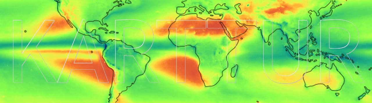
The Vertical Water Balance (VWB) is the local difference between precipitation and evapotranspiration. Regions with precipitation exceeding evapotranspiration are called humid, and areas where evapotranspiration exceed precipitation arid. Many regions have both wet and dry seasons, with humid conditions during the wet season and arid during the dry. Differentiating between humid and arid regions and seasons is important, for instance for understanding and predicting changes in water availability as a consequence of climate changes.

Prerequisites

You must have the complete SPIDE installed as described in the post Install and setup spatial data IDE. You must have setup Karttur’s GeoImagine Framework, either by importing or by copying (drag and drop). The Framework postgres database must be setup and the processes defined. You must also have imported and processed data representing precipitation and evapotranspiration.

Vertical Water Balance

Herein, VWB is calculated as the monthly precipitation minus the monthly evapotranspiration. In this post I use the Tropical Rainfall Measurement Mission (TRMM) dataset together with the FAO reference evapotranspiration (refET) to calculate VWB. To calculate the global VWB you can use the IMERG rainfall dataset instead.

Project module

As explained in the post on Running processes you can create a project module for running specific tasks. The module below links to a single file (VWB_TRMM-vs-FAOrefevap.txt), that in turn links to a set of xml files. Running the module below will run all processes in the listed xml files.

At the very end of the post you find the process chain (i.e. the file VWB_TRMM-vs-FAOrefevap.txt) that will run the complete VWB calculation outlined below; including the time series analysis and export as images and animations.

Preprocessing

Before running the VWB you have to process the precipitation and evapotranspiration data to use as input. Accessing and organizing the TRMM and refET datasets are covered in two previous posts.

Before actually calculating the VWB you must fit the two datasets (rainfall and evapotranspiration) together. For the two datasets used here there are several issues that must be regarded for fitting the datasets:

Units must be the same (e.g mm/month)
The spatial extent must be the same
The spatial resolution must be the same
The regions of nodata should match

The TRMM data was converted to mm/month when imported to the Framework. The FAO reference evapotranspiration data were imported with the original scaling that represent mm/day times 10. Unless you already converted the FAO refET to mm/month, it must be done prior to calculating VWB.

The TRMM dataset covers a smaller spatial region (between 50 degrees latitude) and has a slightly coarser spatial resolution. The easiest way to fit the dataset is thus to reduce the spatial extent and spatial coverage of the FAO reference evapotranspiration. The TRMM data have estimated rainfall for all pixels, including over the oceans. The FAO reference evapotranspiration only covers land. Fitting the datasets should thus also include masking out the same land area.

Adjust the data units

Convert the reference evapotranspiration data in mm/day to mm/month by using the process convertdaytomonth.

Transform the refET

The global refET dataset with monthly average evapotranspiration needs to be fitted to the TRMM dataset. In Karttur’s GeoImagine Framework the process for doing that is gdal_translateancillary. This process is just an interface to the GDAL utility gdal_translate. In the xml file below, the parameters define the translation by setting a pre-defined default region (‘trmm’) and the columns (‘xsize’) and rows (‘ysize’) spanning the default region:

Create a landmask

The FAO refET data only cover land areas. To create a mask, use the transformed version of the refET that fits the TRMM region for defining a mask. You could use any of the months in the refET dataset for defining the mask but to make sure you mask out all regions you can also use all 12 months of refET to define the mask (just to make sure in case there are errors in the FAO refET nodata mask). The process createstaticmaskancillary will do it for you:

Note that the tractid is set to ‘karttur-trmm’, which is the region owned by the user karttur that is based on the default region trmm. When operating on the spatial data, the karttur region ‘karttur-trmm’ will use the default region (‘trmm’) for all naming. This prevents any user (including super users) to operate directly on any default region. A user can only operate on its own regions.

Apply mask

The mask you just created from the refET data must be applied to the complete time series of TRMM rainfall data. This is done with the process applystaticmaskancillary.

Calculate Vertical Water Balance

You should now have two time series covering the same spatial region, with the same spatial resolution and the same area of valid data: the dynamic TRMM precipitation dataset and the statistical FAO refET dataset. You can now calculate the Vertical Water Balance (VWB). As the refET dataset is a statistical seasonal dataset, the calculation of VWB equals removing the seasonal signal from the precipitation time series. As this is water balance data, it can be done in three ways: 1) as the complete difference, 2) only retaining rainfall surplus, or 3) only retaining rainfall deficit. In Karttur’s GeoImagine Framework you can do all three options using the process subtractseasonsancillary.

Resample to annual timestep

To simplify the statistical evaluation and trend analysis, you can translate the data to annual time steps with the process resampletsancillary.

Trend analysis

There are indications that climate change is causing a drying in dry regions/seasons and wetting in wet regions/seasons. To test that you can analyse the overall trends in VWB and compare it with the trends in humid and arid regions. Details about linear trend analysis in Karttur’s GeoImagine Framework is given in the post on SMAP processing. Time series linear trend analysis for ancillary data is done using the process trendtsancillary:

If you want to calculate the trends for other periods (than 1998-2017) you just alter the <period> tag in the xml file.

Change detection

You can use the results from the analysis of VWB trends to identify regions where the change has been significant, and how strong the changes have been. The process for that is signiftrendsancillary

Layout

If you want to create color maps/images and animations for presenting the VWB data you must create the required layout (see post on TRMM for more details).

Set scaling

Layout exports require scaling the original data to byte (0 - 255) range. Details on the scaling are given in the posts on SMAP and TRMM. The xml below calls the scaling definition process createscaling and sets the scaling of both the monthly and annual VWB layers, and all the layers produced as part of the trend analysis.

Add palette

The VWB palettes below, created with the process addrasterpalette, are Karttur’s default palettes for VWB.

Add movieclock

You do not need to add a special movieclock for VWB, the default movieclock works fine. But if you want to create a customised movieclock, the process is addmovieclock. The only parameter that is required is the name of the movieclock, all other parameters are set to default unless explicitly given as parameters (thus the movieclock added below will be identical to the default movieclock).

Export images and create animation

With the scaling and palettes defined, you can export any of the VWB layers created above.

Export monthly images

The full series of monthly VWB images is needed if you want to create an animation. The following xml calls the process exporttobyteancillary and exports all the monthly VWB data, including the overall VWB, the humid VWB and the arid VWB.

Export statistical and trend results

All exports use the same process exporttobyteancillary, you just have to set the timestep and compostions to export all the statistical data, including the results of the trend analysis.

Create movie frames

The process movieframeancillary converts the exported images (from previous step) to movie frames. The process is basically a dimension conversion that can also create an embossed text on the fly. For the process movieframeancillary to work you must have installed imagemagick as explained in another blogpost.

To run the process fully automated you must set the parameter asscript to False, otherwise you must manually execute the shell script file reported when the process comes to an end.

Note that because the three versions of VWB (the total VWB, suplus VWB and deficit VWB) were organized to be stored in the same directory (or folder) path, you can only create one animation at the time. If you want to create animations of all three versions you must delete the “movieframe” folder between each creation.

Create movie clock and animation

The process movieclockancillary first creates the movieclocks to combine with the movie frames from the previous step, and then creates the movie/animation itself. To run the process fully automated you must set the parameter asscript to False, otherwise you must manually execute the shell script files reported when the process comes to an end. By default the process will create script files so you must explicitly enter asscript="False" if you want the process to generate the complete animation on the fly.

For the process <span class=’package’movieclockancillary</span> to work you must have installed FFmpeg as explained in another blogpost.

Process Chain

All of the above processes can be assembled into a single process chain as shown below. To run the process chain you just have to remove the comment marker “#” and run the Framework pointing at the text file with the process chain.