Introduction

SMAP palette

This post introduces processing of data from the Soil Moisture Active Passive (SMAP) mission in Karttur’s GeoImagine Framework. The next post covers defining layouts and exporting the results as different media files. The two following posts deals with capturing SMAP products to the Framework database and how to use SQL to alter the layers to extract from each SMAP products. Then follows a post on how to adjust the SMAP estimates for open water bodies.

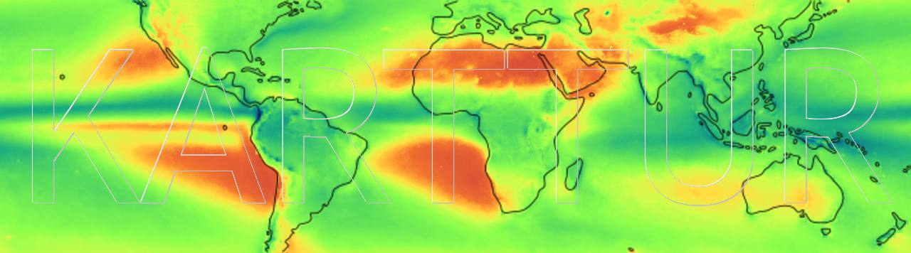
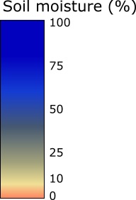
Average soil moisture (vol/vol) for day of year 1 to 16 2015 to 2018. Estimates in arctic regions are derived from interpolation of unfrozen (summer) conditions.

Prerequisites

You must have the complete SPIDE installed as described in the post Install and setup spatial data IDE. You must have setup Karttur’s GeoImagine Framework, either by importing or by copying (drag and drop). The Framework postgres database must be setup and the processes defined.

If you want to use the Framework for searching and registering avaiable SMAP data you must have the terminal command line tool wget (“web get”) installed. Mac osx does not come with wget, you have to install it. I use Homebrew for that:

brew install wget

How to set up Homebrew is covered in this post.

SMAP

The Soil Moisture Active and Passive (SMAP) mission estimates the global top ∼5 cm soil moisture with approximately weekly global coverage. SMAP also determines if the ground is frozen or thawed in colder areas of the world. SMAP was developed for using a combination of active and passive microwave sensors. The active sensor, however, only worked for a couple of months, and the original SMAP combined active and passive data are only available from 13 april to 7 july 2015. Both the active radar and the passive radiometer use the L-band, a microwave frequency that is less disturbed by vegetation and has better ground penetration compared to the more commonly used C-band.

The SMAP passive radiometer original spatial resolution is 36 km, and has been operational since March 2015. Recent algorithmic development has allowed a 9 km enhanced product. Combined with the Sentinel-I active microwave sensor (C-band) a new enhanced active-passive product at 3 km spatial resolution is also under development.

Python Package

The Framework includes a package for specific SMAP processing: geoimagine-smap. The package contains three python modules: smap.py, definetemplate.py and hdf5_2_geotiff.py.

The module definetemplate.py is used for adding records to the SMAP database table on templates. The templates table is required when extracting and organizing SMAP data. The templates define both which layers to extract, how to name them and where to save them. You can accept the default templates that are installed with the GeoImagine Framework database, or you can redefine the database using the definetemplate.py module. You can also check the template definitions, and alter them, by using a graphical interface to the Framework database as described in this post.

SMAP data is projected to an EASE-grid (see below) and the translation of the original hdf data to geotiff requires a special solution available in the module hdf5_2_geotiff.py.

The module smap.py contains all other SMAP specific processing. Note that also several other packages in the Framework are needed for repeating the steps below.

Project module

The project module file (projSMAP.py) is available in the Project package projects.

Process chain

The project file links to an ASCII text file that contains a list of the xml files to execute.

projFN ='doc/SMAP/smap_YYYYMMDD.txt'

As the path to the project file does not start with a slash “/”, the path is relative to the project module itself. The project package available on Karttur’s GitHub page contains the path and the files required for running the process chain. Both the text file and the xml files are available under the subfolder doc/SMAP.

Update DB

The process updatedb is used for transferring database records with associated data processed with the Framework from one computer to another. Examples can be found in the online repository.

Search, download & extract

The SMAP data is available via Alaska Satellite Facility (ASF) and National Snow and Ice Data Center (NSIDC). The higher level products (used in this post) are only available from NSIDC. To get access to the data hosted by NSIDC you must sign up with https://earthdata.nasa.gov.

Searching the SMAP online repository

The way Karttur´s GeoImagine Framework is organized, you first have to search the online repository, then register the search results in the Framework postgres database. Once the data is registered you can download and extract the actual SMAP data.

Search

I have tried to find some library or database that lists the data available in the online repositories, but have failed to find any. Instead I created a solution where I use wget (“web get”) for downloading an html coded list of available data. For more information on wget, see the Prerequisites above. The Framework process for searching the online repository for SMAP data using wget is SearchSmapProducts.

The project xml folder (doc/SMAP/xml) contains a number of xml files for searching the online database. If the end date is set to a date later than today, the search will stop at todays date and thus you can safely put a future date to be sure to get all the recent data.

Before running the process SearchSmapProducts you must have the credentials for accessing https://earthdata.nasa.gov in a .netrc file, with the username corresponding to the one given in the xml file (‘YourEarthDataUser’). The use of .netrc for accessing protected sites is introduced in this post.

The process SearchSmapProducts. drills into https://earthdata.nasa.gov and loads the available files as html code. By default the process saves one html file per date (online sub-folder) under the path ../smap/source/yyyy.mm.dd/ (where yyyy.mm.dd is the date of acquisition) on the volume identified in the xml file. The files are ordinary html files, but with the .html extension omitted.

Active Passive (2015)

The active Synthetic Aperture Radar (SAR) instrument was only operational for a few months in 2015.

Passive 2015 - 2018

The passive radiometer instrument has been continuously operating since March 2015. To facilitate updating the processing is divided between “past” (only needs to be done once) and “present”,

Passive 2019 to present

Transfer search to database

To transfer the search results to the GeoImagine Framework database you must run the process SmapSearchToDB. It reads the html files created by SearchSmapProducts, extracts the required information and inserts the information in the database. When finished it moves the html file to a sub-folder called done. If, for some reason, you delete your database all you need to do is to take all the html files under the done sub-folder and move them one level up and then re-run SmapSearchToDB.

Active Passive data

Passive data 2015 - 2018

Passive data 2019 to present

Downloading SMAP data

With the available SMAP data registered in the database you can download any of the registered data using the process DownLoadSmapDaac.

I have tried to figure out how to extract individual layers from the SMAP online repository HDF5 files. But I have not managed. Hence the process DownLoadSmapDaac will always download the complete HDF5 files for each product and date. For most of the products this is really not a problem, but the recently available enhanced products can be very large.

When downloading the SMAP HDF5 files you can either download the files on the fly, or write the download commands to a shell script file. The latter is the default. To change it you need to set the parameter asscript to False.

If you did not add the parameter asscript, including setting it to False, the process produces a script file that you must run manually. You can also copy the script to another machine (with better internet connection) and run the script from there. The machine you run from must have a .netrc file with your EarthData credentials. And the volume indicated in the xml must either exists on the machine from which you download, or you need to edit the script to reflect a volume that is available on the machine from which you download. To run the shell script you must first make it executable, and then execute it:

$ chmod 777 /path/to/script.sh

$ /path/to/script.sh

Active Passive data

Passive data 2015 - 2018

Passive data 2019 to present

Registering Downloads

If you downloaded SMAP data on the fly (i.e. with parameter asscript set to False), your downloads are automatically registered in the database. If you downloaded via script they are not. The easiest way to register the downloads is to re-run DownLoadSmapDaac with the same parameters (xml command file) and the script will recognize that the SMAP tiles are already downloaded and register them.

Extract SMAP layers

The layers included in each HDF5 file, as well as metadata, can be accessed using gdalinfo.

gdalinfo /path/to/smap/hdf5file.H5

In Karttur’s GeoImagine Framework the layers to extract have to be defined in the database, in the table templates under the smap schema. The template table also define the celltype, cellnull, projection and folder where to store the extracted layer. The two following posts deals with how to fill and edit the table smap.temaplates. To extract the layers run the process extractSmapHdf, but first a bit of information on the SMAP data projection.

The EASE-Grid projection

The SMAP data are projected using the equal area EASE-Grid 2.0 projection, using three different regions:

A global cylindrical EASE grid (EPSG:6933)
A northern polar EASE grid (EPSG:6931)
A southern polar EASE grid (EPSG:6932)

As with all other data imported to Karttur’s GeoImagine Framework, the basic projection is kept, and only changed when data from different systems are combined (i.e. you can combine SMAP with MODIS by transferring the SMAP data to fit MODIS sinusoidal grids).

It is best to use the EPSG code when working with the SMAP data. The EASE-Grid 2.0 projection requires that proj4 is at least version 4.8. You need to check that out. If you have an earlier version of proj4, you can use the proj4 definition instead of the EPSG code:

+proj=cea +lon_0=0 +lat_ts=30 +x_0=0 +y_0=0 +ellps=WGS84 +towgs84=0,0,0,0,0,0,0 +units=m +no_defs

If you look in the module hdf5_2_geotff.py, you can alter between defining the projection using proj4 and the EPSG code. If you are not sure, please use the full proj4 definition above instead of the EPSG code.

The process extractSmapHdf extracts the layers defined in the database from the HDF5 files.

The process identifies missing HDF5 files on the fly, and create a shell script file that, if executed, will download the missing files. Thus you have to give your remote user for EarthData. If you do not have any user for EarthData you can enter any text string for the extraction itself.

Active Passive data

Passive data 2015 - 2018

Passive data 2019 to present

Overlay special

The daily data for most SMAP L3 products are separated into morning (am) and evening (pm) observed soil moisture. And the extraction above will in general produce both am and pm layers. To create daily average (or minimum or maximum) composites use the Framework process conditionaloverlay. It ignores “null” when overlaying data, and for creating the daily average that is what you want.

Overlay am and pm to daily average

SMAP palette

The overlay of am and pm data to daily averages as defined in the xml commands below are done for several of the sub-datasets of the different SMAP products.

Daily SMAP maps for the 22 January 2016. The left image is the morning (am) soil moisture, the right image is the afternoon (pm) soil moisture and the central image is a combination of the other two.

Time series processing

For some of the analysis and modeling the daily timestep is the best solution. But for comparison with e.g. climate data, vegetation growth, or other satellite images like MODIS, the SMAP data need to be aggregated. This also has the advantage that if you aggregate to weekly data, or more, you will get estimates with total global coverage (not strips like in the figure above).

Temporal resampling

A lot of the processing examples in this blog rely on weekly to biweekly, or monthly timesteps. MODIS products typically represent 8 or 16 day intervals, the old crop-climate data from AVHRR images usually come as three (3) monthly periods, and a lot of climate data is available using monthly aggregated data.

The temporal frequencies defined in Karttur’s GeoImagine Framework rely on the Pandas package. Pandas is widely used for handling time series data in Python, and is part of Anaconda (the python distribution used by Karttur´s GeoImagine Framework). It can be a bit slow to use for resampling, and for some of the resampling the GeoImagine Framework instead use numba JIT (Just In Time) compiled scripts. But the frequency definitions and conversions rely on Pandas.

The Framework process for temporal aggregation (resampling) of SMAP data is resampletssmap.

Resampling 16 day intervals

To resample SMAP from daily to 16 day intervals (same temporal resolution as several MODIS products) set the parameter targettimestep to 16D (as shown in the xml example below). The start date given in the period tag will determine the start and end date of each 16D period. You can create a gliding mean of the 16D interval by repeating the process 16 times, each time with a 1 day difference of the starting date. The setting below will cause the 16D interval to coincide with The MODIS 16D standard intervals.

Opening and processing daily SMAP data covering a temporal span of multiple years demands a lot of computer power, and for that reason I have divided the resampling into annual steps. I thus resample each individual year separately. The result is the same as resampling the whole time series in one go, but is less memory intense. The example below shows the resampling of the incomplete start year for SMAP (2015). All other years are available in the online project xml folder. Note hoe the enddate is set to 10 January 2016. This is required in order to capture the complete 16 day period centering on the last 16 day period in 2015.

Average soil moisture (vol/vol) for days 1 to 16 in 2016.

Resampling to monthly intervals

The xml example below shows how to resample the daily SMAP values to monthly average. The example is for a year with complete data (2016).

Seasonal signal extraction

The process extractseasonsmap extracts the seasonal multiyear signal. The extraction can be set to force interpolation of all seasons lacking data. For the SMAP soil moisture data all frozen soils lack estimates of soil moisture, and the soil moisture conditions under frozen soil are force-filled by interpolation for all pixels. This is an oversimplification, but also has advantages; including when presenting the data, like in the animations below.

Extract 16D seasonal signal

The process extractseasonsmap uses all data available within the defined period for retrieving a seasonal signal. In the example below the 16D seasonal cycle is extracted using all dates between 23 April 2005 and 19 February 2019. The process can be set to linearly interolate any missing season.

Extract monthly seasonal signal

Interpolate nodata considering seasonal signal

Karttur´s GeoImagine Framework provides some different methods for interpolating time series data and force fill all periods. The simplest method is to do a linear interpolation, as used for filling in missing data for e.g. GRACE. The more advanced method is to use a nonlinear interpolation and also adjust for the seasonality. This requires that you first extract the seasonal signal for the same period you want to interpolate (as in the step above), then you can apply the process seasonfilltsSmap. The processes applies a weighted linear interpolation giving larger weight to the previous observation compared to the next, while also including the seasonal signal. At small gaps (a single missing date) the seasonal signal is almost irrelevant; the larger the gap the larger the influence of the seasonal signal.

Interpolate nodata for 16D time series

Resources

Karttur´s GeoImagine Framework

the EASE-Grid Projection by NSIDC

hdf5_to_geotiff GitHub script for projecting SMAP layers in EASE-Grid 2