You must have completed the data processing of GRACE data in the previous post.
GRACE
Project module
The project module file (projGRACE.py) is available in the Project package projects.
from geoimagine.kartturmain.readXMLprocesses import ReadXMLProcesses, RunProcesses

if __name__ == "__main__":

    verbose = True

    projFN ='doc/GRACE/grace_20190216.txt'
    projFN ='doc/Layout/grace-layout_20190216.txt'

    procLL = ReadXMLProcesses(projFN,verbose)

    RunProcesses(procLL,verbose)
Process chain
The project file links to an ASCII text file that contains a list of the xml files to execute. The layout and export processes are under the folder Layout.
projFN ='doc/Layout/grace-layout_20190216.txt'
As the path to the project file does not start with a slash “\”, the path must be relative to the project module itself. The project package available on Karttur’s GitHub page contains the path and the files required for running the process chain.
###################################
###################################
###            GRACE            ###
###################################
###################################

###################################
###            Layout           ###
###################################

## Create scaling for GRACE compids ##
GRACE-0001_createscaling.xml

## Create palettes for GRACE ##
GRACE-0002_createpalettes.xml

## Create legend for GRACE ##
GRACE-0003_createlegends.xml

## Export legends for GRACE ##
GRACE-0005_exportlegend.xml

## Create movie clock ##
#smap_createmovieclock.xml

###################################
###        Export media         ###
###################################

## Export graticule as svg ##
#GRACE-0925_graticule_ExporttoSVG.xml

## Export annual statistics, trends and changes ##
#GRACE-0910_ExporttoByte_timespanA_2003-2016.xml
Layout
To produce a color map, you need to scale your original map to range between 0 and 250 (or lower), and then assign the palette. To create and export a layout map or image, you must pre-define the scaling for the composition to export. All exported images (maps) are scaled to Byte range (0 to 255), and the scaling should achieve that while preserving a relevant distribution of numerical cell values. By default, the Framework assumes that null (nodata) will equal 255 in the scaled export, and that the values 251 to 254 represent colors for overlays, frames and text etc. Values in the range 0 to 250 (or lower) should represent the thematic feature of the layer.
Scaling
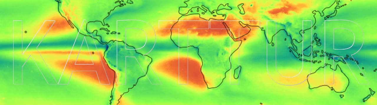
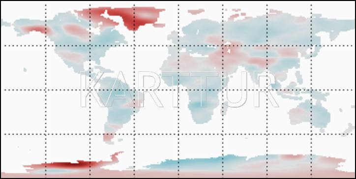
The GRACE data is strongly skewed because of the glacier melt in Greenland and West Antarctica. The melting of the glaciers causes a loss in water and thus gravitational pull. Using a linear scale for representing the global change in water equivalent thickness that include the melting glacier thus becomes tricky. I choose to use a solution with a power function to capture both large and small changes. This, however, can be deceptive but you need to choose some legend scaling in order to show your map. The process createscaling adds the scaling to the database.
If you want to produce color maps showing the GRACE data and the results of your trend analysis, you also need to create the palette(s) to use. All palettes must be saved to the database before use, with the process addrasterpalette. Glancing at the color ramp of the online GRACE data at the official homepage, I set the following palette:
<?xml version='1.0' encoding='utf-8'?>
<palette>
<userproj userid = 'karttur' projectid = 'karttur' tractid= 'karttur' siteid = '*' plotid = '*' system = 'system'></userproj>
<path></path>


<!-- addrasterpalette preciplinear-->
<process processid = 'addrasterpalette'>
<overwrite>Y</overwrite>
<delete>N</delete>
<parameters palette = 'grace' compid='test'>
<setcolor id = '0' red = '96' green ='0' blue='0' alpha ='0' label='0' hint='0' ></setcolor>
<setcolor id = '63' red = '204' green ='74' blue='70' alpha ='0' label='25' hint='NA' ></setcolor>
<setcolor id = '125' red = '224' green ='224' blue='224' alpha ='0' label='50' hint='50' ></setcolor>
<setcolor id = '187' red = '60' green ='170' blue='190' alpha ='0' label='75' hint='NA' ></setcolor>
<setcolor id = '250' red = '4' green ='4' blue='110' alpha ='0' label='100' hint='100' ></setcolor>
<setcolor id = '253' red = '240' green ='240' blue='132' alpha ='0' label='dry (0)' hint='NA' ></setcolor>
<setcolor id = '254' red = '32' green ='32' blue='32' alpha ='255' label='frame' hint='frame' ></setcolor>
<setcolor id = '255' red = '250' green ='250' blue='250' alpha ='255' label='255' hint='no data' ></setcolor>
</parameters>
</process>


</palette>
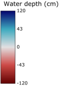
Create Legend
The process createlegend defines the legend layout for compositions. When producing the legends the colors and denominations of the actual legend items are taken from the definition of palettes and scalings respectively.
<?xml version='1.0' encoding='utf-8'?>
<palette>
<userproj userid = 'karttur' projectid = 'karttur' tractid= 'karttur' siteid = '*' plotid = '*' system = 'system'></userproj>


<!-- Create legend -->

<!-- NOTE THE ID IS OLNLY USED IN THE SCRIPTING SO IT CAN HAVE (UNIQUE) DUMMY VALUES HERE -->
<!-- GRACE monthly cmwater-->
<process processid = 'createlegend' version = '1.3'>
<overwrite>True</overwrite>
<parameters columnhead='Water depth (cm)' precision='0'></parameters>
<comp id = '1' source = "NASA-GRACE" product = "ave-cmwater" folder = "cmwater-annual-stats-A" band = 'avg-grace-ave' suffix = "RL05-filled"></comp>
</process>

<!-- GRACE annual average cmwater-->
<process processid = 'createlegend' version = '1.3'>
<overwrite>True</overwrite>
<parameters columnhead='Water depth (cm)' precision='0'></parameters>
<comp id = '1' source = "NASA-GRACE" product = "ave-cmwater" folder = "cmwater-annual-stats-A" band = 'avg-grace-ave' suffix = "RL05-filled"></comp>
</process>

<!-- GRACE annual std cmwater-->
<process processid = 'createlegend' version = '1.3'>
<overwrite>True</overwrite>
<parameters columnhead='Water depth (cm)' precision='0'></parameters>
<comp id = '1' source = "NASA-GRACE" product = "ave-cmwater" folder = "cmwater-annual-stats-A" band = 'std-grace-ave' suffix = "RL05-filled"></comp>
</process>

<process processid = 'createlegend' version = '1.3'>
<overwrite>True</overwrite>
<parameters columnhead='MK test (Z-value)'></parameters>
<comp id = '1' source = "NASA-GRACE" product = "ave-cmwater" folder = "cmwater-annual-trend-A" band = 'mk-z-grace-ave' suffix = "RL05-filled"></comp>

</process>

<process processid = 'createlegend' version = '1.3'>
<overwrite>True</overwrite>
<parameters columnhead='Rainfall trend:(mm/yr)' precision='0'></parameters>
<comp id = '1' source = "NASA-GRACE" product = "ave-cmwater" folder = "cmwater-annual-trend-A" band = 'ts-mdsl-grace-ave' suffix = "RL05-filled"></comp>
</process>

<process processid = 'createlegend' version = '1.3'>
<overwrite>True</overwrite>
<parameters columnhead='Rainfall trend:(mm/yr)' precision='0'></parameters>
<comp id = '1' source = "NASA-GRACE" product = "ave-cmwater" folder = "cmwater-annual-trend-A" band = 'ts-hisl-grace-ave' suffix = "RL05-filled"></comp>
</process>

<process processid = 'createlegend' version = '1.3'>
<overwrite>True</overwrite>
<parameters columnhead='Rainfall trend:(mm/yr)' precision='0'></parameters>
<comp id = '1' source = "NASA-GRACE" product = "ave-cmwater" folder = "cmwater-annual-trend-A" band = 'ts-losl-grace-ave' suffix = "RL05-filled"></comp>
</process>

<process processid = 'createlegend' version = '1.3'>
<overwrite>True</overwrite>
<parameters columnhead='Rainfall (mm)' precision='0'></parameters>
<comp id = '1' source = "NASA-GRACE" product = "ave-cmwater" folder = "cmwater-annual-trend-A" band = 'ts-ic-grace-ave' suffix = "RL05-filled"></comp>
</process>

<process processid = 'createlegend' version = '1.3'>
<overwrite>True</overwrite>
<parameters columnhead='Rainfall trend:(mm/yr)' precision='0'></parameters>
<comp id = '1' source = "NASA-GRACE" product = "ave-cmwater" folder = "cmwater-annual-trend-A" band = 'ols-sl-grace-ave' suffix = "RL05-filled"></comp>
</process>

<process processid = 'createlegend' version = '1.3'>
<overwrite>True</overwrite>
<parameters columnhead='Correlation (r2)' palmax='100'></parameters>
<comp id = '10' source = "NASA-GRACE" product = "ave-cmwater" folder = "cmwater-annual-trend-A" band = 'ols-r2-grace-ave' suffix = "RL05-filled"></comp>
</process>

<process processid = 'createlegend' version = '1.3'>
<overwrite>True</overwrite>
<parameters columnhead='Rainfall (mm)' precision='0'></parameters>
<comp id = '11' source = "NASA-GRACE" product = "ave-cmwater" folder = "cmwater-annual-trend-A" band = 'ols-rmse-grace-ave' suffix = "RL05-filled"></comp>
</process>

<process processid = 'createlegend' version = '1.3'>
<overwrite>True</overwrite>
<parameters columnhead='Rainfall (mm)' precision='0'></parameters>
<comp id = '12' source = "NASA-GRACE" product = "ave-cmwater" folder = "cmwater-annual-trend-A" band = 'ols-ic-grace-ave' suffix = "RL05-filled"></comp>
</process>

<process processid = 'createlegend' version = '1.3'>
<overwrite>True</overwrite>
<parameters columnhead='Rainfall change:(mm)' precision='0'></parameters>
<comp id = '13' source = "NASA-GRACE" product = "ave-cmwater" folder = "cmwater-annual-trend-A-model" band = 'delta-grace-ave' suffix = "RL05-filled"></comp>
</process>

<process processid = 'createlegend' version = '1.3'>
<overwrite>True</overwrite>
<parameters columnhead='Rainfall change:(mm)' precision='0'></parameters>
<comp id = '14' source = "NASA-GRACE" product = "ave-cmwater" folder = "cmwater-annual-trend-A-model" band = 'mk-ts-mod@p005-grace-ave' suffix = "RL05-filled"></comp>
</process>

<process processid = 'createlegend' version = '1.3'>
<overwrite>True</overwrite>
<parameters columnhead='Rainfall change:(mm)' precision='0'></parameters>
<comp id = '15' source = "NASA-GRACE" product = "ave-cmwater" folder = "cmwater-annual-trend-A-model" band = 'mod@p005-2003-grace-ave' suffix = "RL05-filled"></comp>
</process>

<process processid = 'createlegend' version = '1.3'>
<overwrite>True</overwrite>
<parameters columnhead='Rainfall change:(mm)' precision='0'></parameters>
<comp id = '16' source = "NASA-GRACE" product = "ave-cmwater" folder = "cmwater-annual-trend-A-model" band = 'mod@p005-2016-grace-ave	' suffix = "RL05-filled"></comp>
</process>
</palette>
Export legend
With the process exportlegend you can create stand alone legends. To work you mtust have defined the scaling, the palette and the legend in the previous steps. The process produces two legends, as a Scalable Vector Graphics (.svg file) and a .png file. The svg is saved as a www compliant xml, and you can use it either for editing in a graphics program or inclusion in a web-page (or both).
<?xml version='1.0' encoding='utf-8'?>
<exportlegend>
<userproj userid = 'karttur' projectid = 'karttur' tractid= 'karttur' siteid = '*' plotid = '*' system = 'system'></userproj>


<!-- Export legend -->

<!-- NOTE THE ID IS OLNLY USED IN THE SCRIPTING SO IT CAN HAVE (UNIQUE) DUMMY VALUES HERE -->
<!-- GRACE monthly cmwater-->
<process processid = 'exportlegend' version = '1.3'>
<overwrite>True</overwrite>
<parameters palette='grace'></parameters>
<dstpath volume='karttur3tb'></dstpath>
<comp id = '1' source = "NASA-GRACE" product = "ave-cmwater" folder = "cmwater-annual-stats-A" band = 'avg-grace-ave' suffix = "RL05-filled"></comp>
</process>

</exportlegend>
Export overlay
When you export the actual data as maps in the next step, you can add a vector overlay. In the Framework you can convert any vector to an svg and then include it as an overlay. Only a single svg file can be used as overlay when exporting raster data to image maps. But you can manually compose an svg from multiple svg exported vectors, e.g. using a graphics editor.
For the GRACE data a graticule is exported from a vector file including longitude and latitude lines for each 45 degrees.
Having defined the scaling and a palette for the different layers, you can export the layers as color maps (colored GeoTiff images). The process for doing that is exporttobyteancillary.
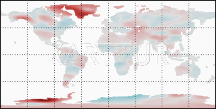
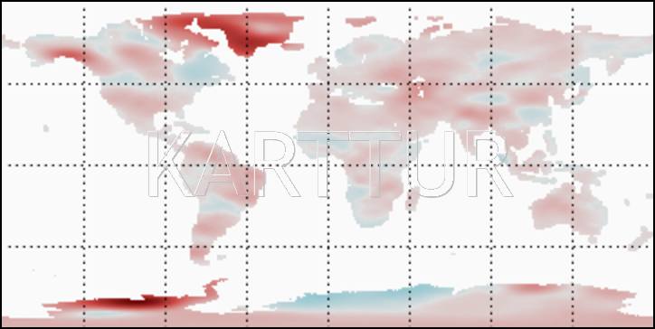
Maps of the change in water equivalent thickness 2003 to 2016. The top row shows the Ordinary Least Square (OLS) slope and the Theil-Sen (TS) median slope. The bottom row shows the lower and higher 95 % confidence limit for TS slope.