GRACE was built around two identical satellites orbiting the Earth and was operational from 2003 to 2017. Traveling with a fixed distance in between them the gravitational pull caused minute changes in the vertical elevation difference between the two satellites. This change can be used for estimating the gravitational pull. Short term (days to months) changes in the gravitation over land is primarily related to the Earth’s water reservoirs, earthquakes and crustal deformations.
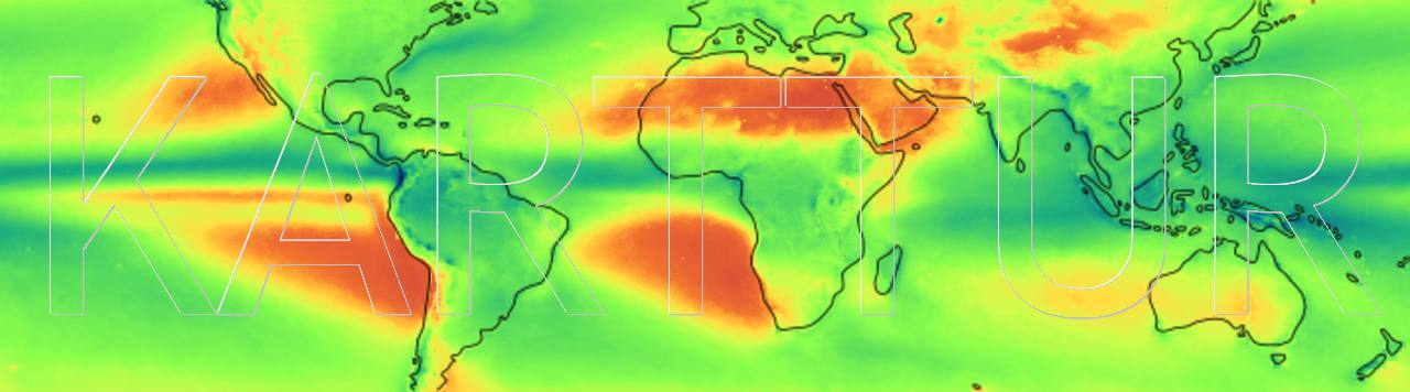
This tutorial makes use of GRACE TELLUS Level-3 data grids of monthly surface mass changes to detect trends in water storage on land. This GRACE data represent the changes in equivalent water thickness relative to a (time-mean) baseline. There are three different solutions for the calculations of equivalent water thickness, respectively produced by CSR (Center for Space Research at University of Texas, Austin), GFZ (GeoforschungsZentrum Potsdam) and JPL (Jet Propulsion Laboratory). You can use any of these solutions, but the official recommendation is that users obtain all three data center’s solutions (JPL, CSR, GFZ) and simply average them.
Python Package
The GeoImagine Framework includes a specific package for GRACE processing: grace. Note that also several other packages in the Framework are needed for repeating the steps below.
Project module
The project module file (projGRACE.py) is available in the Project package projects.
from geoimagine.kartturmain.readXMLprocesses import ReadXMLProcesses, RunProcesses

if __name__ == "__main__":

    verbose = True

    projFN ='doc/GRACE/grace_YYYYMMDD.txt'

    procLL = ReadXMLProcesses(projFN,verbose)

    RunProcesses(procLL,verbose)
Process chain
The project file links to an ASCII text file that contains a list of the xml files to execute.
projFN ='doc/GRACE/grace_20181018_0.txt'
As the path to the project file does not start with a slash “/”, the path must be relative to the project module itself. The project package available on Karttur’s GitHub page contains the path and the files required for running the process chain. Both the text file and the xml files are available under the subfolder doc/GRACE.
###################################
###################################
###            GRACE            ###
###################################
###################################

###################################
###     Download & organize     ###
###################################

## The GRACE mission is finished and the data must be
## manually searched and downloaded as described in the
## SMAP blogpost: https://karttur.github.io/geoimagine/blog/blog-SMAP/

## Organize the downloaded GRACE data ##
#GRACE-0101_organize.xml

## Mend GRACE by interpolating missing dates ##
#GRACE-0111_mendts.xml

## Average the three GRACE solutions ##
#GRACE-0115_average.xml

## Convert month format to karttur standard ##
#GRACE-0120_monthdaytomonth.xml

## Alternative import pre-processed GRACE data and update db ##
#GRACE-0190_updatedb.xml

###################################
###   Time series processing    ###
###################################

## Extract GRACE seasonal signal ##
#GRACE-0231_extract-season.xml

## Resample Grace to Annual ##
GRACE-0290_resample-2-annual.xml

## Estimate trend from annual timestep ##
#GRACE-0310_trend_A_2003-2016.xml

## Calculate annual changes 2003 t0 2016 ##
#GRACE-0320_changes_A_2003-2016.xml
Import pre-processed GRACE data and update db
If you already got access to GRACE data produced with Karttur´s GeoImagine Framework you can use the process updatedb to import the data to your Framework.
In the example above the imported layers represent the nodata-filled and averages solution for mm water pillar. The next step with this import would then be the time series processing.
Download & organize
THe GRACE data is freely available from GRACE TELLUS. The data are available through ftp, and the dataset is small and the experiment finished. The easiest way to download the data is to use an FTP client (for example Filezilla).
The data can be downloaded as NetCDF files, as GeoTIFF images and as ASCII text files. Karttur’s GeoImagine Framework can import any of these formats, but the specific GRACE importer that solves the projection of the GRACE data on the fly use the ASCII data as input. When downloading the data, make sure to keep the same folder structure as the online resource (this is how the import process expects the data).
Organizing the dataset
The GRACE dataset available online is not projected in the usual manner; the left edge starts at the Greenwich Meridian and then extends eastwards. It wraps the dateline and the last column again ends at the Greenwich Meridian. To solve the projection on the fly when organizing GRACE data, use the process OrganizeGrace (only works on the ASCII data). This process is a subclass to OrganizeAncillary, and uses the same xml structure:
The process OrganizeGrace translates the raw GRACE data to organized and projected GeoTIFF layers. The xml does not define the layers explicitly. Like for all processes, the spatial data is defined by a compositon object, a region (tract, site or plot) and a time span inculding a temporal resolution. When the process is exectuted the layers are constructed from a compostion, a loaction and a time stamp.
In the xml above, the region is defined by the tract:
tractid= 'karttur'
Where the tractidkarttur is the default superuser owned tract representing global extent (see this post for details).
The time span and the temporal resolution is defined in the <period> tag:
<period timestep='allscenes'></period>
The timestep parameter allscenes only works for some processes; for GRACE data it searches the source data for all available data found under the import path.
The composition is completely defined by the following tag:
You can change the composition definition to anything you want, but you must define all parameters.
If you want to use all the solutions for equivalent water thickness (CST, GFZ and JPL) you have to define three import processes (can be done in the same xml file).
Filling missing data
The GRACE monthly dataset of equivalent water thickness has some gaps. The process mendancillarytimeseries fills the gaps. The default method for filling data is linear interpolation. Note that the <srccomp> tag in the xml below is identical to the <dstcomp> tag in the xml defining the import (above). In the xml file below also the time period and the temporal resolution are explicitly defined.
As note above, the recommendation is to use the average of the three solutions for the monthly equivalent water depth (CSR, GFZ and JPL). The process average3ancillarytimeseries will do this for you. You must have imported and filled all three solutions (the process source datasets).
The date format of the downloaded GRACE data is YYYYMM01, where YYYY is the year and MM the month. The data, however, does not represent the 1st day of the denoted month but the average for the whole month. In Karttur´s GeoImagine Framework, data representing a month is given as YYYYMM (see this post). The process monthdaytomonth converts the GRACE data date format to the Framework standard.
The process extractseasonancillary extracts the seasonal mean for each season in the dataset (monthly periods for the GRACE data). This process is not needed for the analysis of the GRACE data as done in this post.
In this example we are just going to look at the annual changes in water equivalent depth using the GRACE data. To do that you must resample the monthly data to an annual signal. The process for this is resampletsancillary
For the GRACE data, that describes the relative change, it does not really matter if you resample using the average annual signal or sum up the monthly signals to an annual sum. In the example I have resampled to annual average.
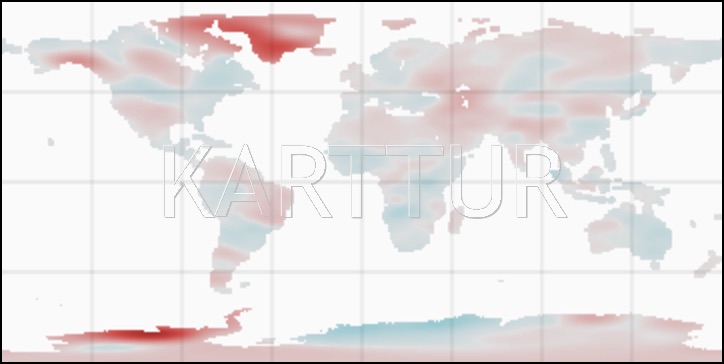
In this example the trend of the changes in equivalent water thickness will be done using the annual average GRACE data. The process for this is trendtsancillary. At time of writing, it can use two different linear methods for estimating the trend: Ordinarly Least Sqaure (OLS) and Theil-Sen (TS). For determining the significance of the change in the linear trend the process uses the Mann-Kendall (MK) test. The script is set up so that you just state ols or mk (or both), the additional analysis follow along. With ols given you also get the random mean square error (‘rmse’) and the correlations coefficient (‘r2’), and with mk you get the TS regression (median and at 95 % confidence limits for upper and lower change). The script can also calculate the long term average and standard deviations. The xml parameters below generate all the output options presently available:
The process signiftrendsancillary combines the MK test with the TS slope and estimates the absolute changes over the defined period. Two layers are produced, one showing the changes for all areas, and one showing only areas with statistically significant changes.