Introduction

This post illustrates how to use Karttur’s GeoImagine Framework for calculating autocorrelation in image time series data.

Prerequisites

You must have setup the Karttur’s GeoImagine Framework as described in earlier posts. You must also have created the monthly TRMM rainfall dataset from scratch, or imported from pre-processed data. Alternatively you can use any other time series dataset with regular (e.g. monthly) intervals, for example GRACE, or resampled SMAP data.

Autocorrelation

The autocorrelation of a time series reveals how the signal at a given time correlates with the signal at different lags (or later times). This allows for a better understanding of (seasonal) signal patterns and the temporal dependencies. This information can be used both for adjusting the time series data and for improving forecast models.

Framework process

The process for analysing autocorrelation in Karttur’s GeoImagine Framework is autocorrelate. The autocorrelation can be set to either a full autocorrelation function (acf) or a partial acf (pacf) as defined in the statsmodel package.

XML commands

The example below shows how to run acf (default) for a time series of 20 years on monthly TRMM rainfall data. The number of lags (nlags) to compute must be given. If mirror is set, the integer value will be used for adjusting seasonality to an annual cycle and the nlags should be set to the total number of season (i.e. 12 for monthly data).

Hide/Show TRMM041_autocorrelate_M_v80.xml

  
<?xml version='1.0' encoding='utf-8'?>
<autocorr>
	<userproj userid = 'karttur' projectid = 'karttur' tractid= 'karttur-trmm' siteid = '*' plotid = '*' system = 'ancillary'></userproj>
	<period startyear = "1998" startmonth='01' endyear = "2017" endmonth='12' timestep='M'></period>

	<process processid = 'autocorrelateancillary' version = '1.3'>
		<overwrite>Y</overwrite>
		<parameters nlags = '12' partial='False' resampleseasonal='False' mirror ='6' ></parameters>
		<srcpath volume = "karttur3tb" hdrfiletype = 'tif' datfiletype = 'tif'></srcpath>
		<dstpath volume = "karttur3tb" hdrfiletype = 'tif' datfiletype = 'tif'></dstpath>
		<srccomp>
			<trmm-3b43v7-precip  source = "trmm" product = "3b43" folder = "rainfall" band = "trmm-3b43v7-precip" prefix = "rainfall" suffix = "v7-f">
			</trmm-3b43v7-precip>
		</srccomp>
	</process>
</autocorr>

Results

The process autocorrelate generate one layer per lag up to the number of requested lags. If mirror is set to a number larger than zero, negative numbers in the file date part indicates the correlations with the prior period.

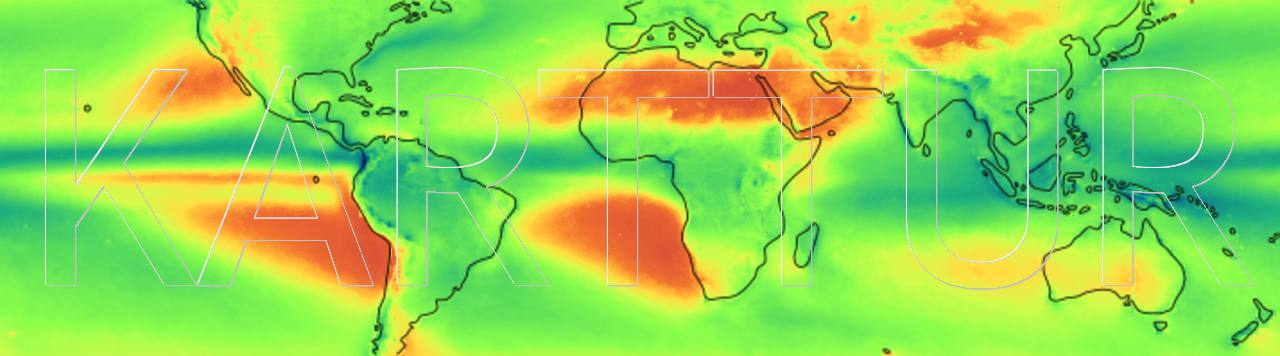
Figure X shows the global autocorr for ???