Introduction

Cross correlation is a measure of similarity between two (time) series given a lag (or displacement) of one relative to the other. In some cases one of the series can be regarded as a driver (e.g. rainfall) and the other as a slave (e.g. soil moisture or vegetation growth). Cross correlation is similar to auto correlation, but instead of finding the correlation in a single time series, cross correlation compares two time series while changing the lag time.

In Karttur’s GeoImagine Framework, cross correlation is tested using the same principles as in numpy.crosscorr, but with the customized code by Jean-Rémi King available on GithHub. The difference is that the latter code allows the setting of a maximum number of lags, and is thus faster compared to the former.

All cross correlations report two results: the lag and the Pearson correlation number for the best fitted lag.

Overview

In this tutorial you will test cross correlation in Karttur’s GeoImagine Framework by comparing times series of a climate index with the time series of local TRMM rainfall. Both of these time series have the same monthly temporal resolution. The climate index can also be regarded as a driver of the local rainfall. You can choose any location to work with, but if you want to study the correlation at latitudes above 50 degrees you have to use IMERG rainfall dataset instead of TRMM.

The cross correlation between the climate indexes and local rainfall is of interest for explaining variations in both seasonal patterns, long term trend or tendency, and unexplained local variations (as defined from time series decomposition).

Prerequisites

You must have setup the Karttur’s GeoImagine Framework as described in earlier posts. You must also have added the climate indexes to the database and imported the TRMM rainfall and/or IMERG rainfall datasets.

Framework process

To illustrate how the cross correlation works, you will use the Framework package for plotting cross correlations between an index and an image time series indexcompxcrosstsgraphancillary. There are many options for parameterizing this package and only a few options will be explored in the tutorial. If you go to the process page you can see all options.

Process commands

Default setting

By default the indexcompxcrosstsgraphancillary analyses the cross correlation only for the original (observed) time series. You can state as many locations (<xy >) to compare as you like, but only one climate index.

<?xml version='1.0' encoding='utf-8'?>
<crosscorrplot>
	<userproj userid = 'karttur' projectid = 'karttur' tractid= 'karttur-trmm' siteid = '*' plotid = '*' system = 'ancillary'></userproj>
	<period startyear = "1998" startmonth='01' endyear = "2017" endmonth='12' timestep='M'></period>

	<process processid = 'indexcompxcrosstsgraphancillary' version = '1.3'>
		<parameters
		></parameters>
		<srcpath volume = "karttur3tb" hdrfiletype = 'tif' datfiletype = 'tif'></srcpath>
		<dstpath volume = "karttur3tb" hdrfiletype = 'tif' datfiletype = 'tif'></dstpath>
		<srccomp>
			<trmm-3b43v7-precip  source = "trmm" product = "3b43" folder = "rainfall" band = "trmm-3b43v7-precip" prefix = "rainfall" suffix = "v7-f">
			</trmm-3b43v7-precip>
		</srccomp>
		<xy id ='Okavango' x='35' y='-22' obscolor = 'b' tendencycolor = 'b'  seasoncolor = 'b' residualcolor = 'b'></xy>
		<xy id ='Lake Victoria' x='35' y='0' obscolor = 'g' tendencycolor = 'g'  seasoncolor = 'g' residualcolor = 'g'></xy>
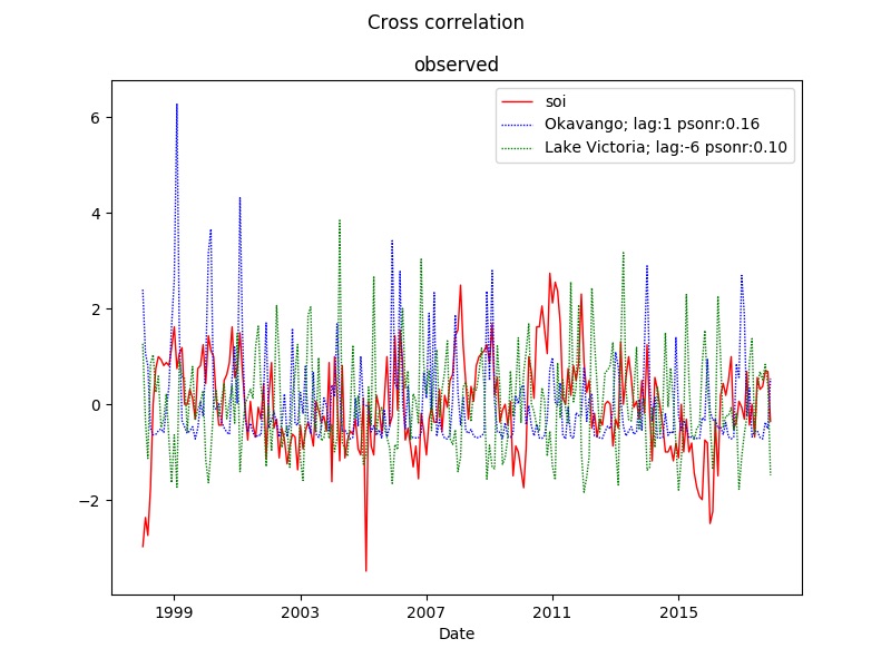
		<index id='soi' obscolor = 'r' tendencycolor = 'r' seasoncolor = 'r' residualcolor = 'r'></index>
	</process>
</crosscorrplot>

The figure below illustrates the results for the xml parameterization above, but with the left figure only showing one (Okavango) of the positions (psonr = pearson number).

Cross correlation between the Southern Oscillation Index (SOI) and local rainfall at Okavango (Botswana) and Lake Victoria (Uganda).

Cross correlation with time series components

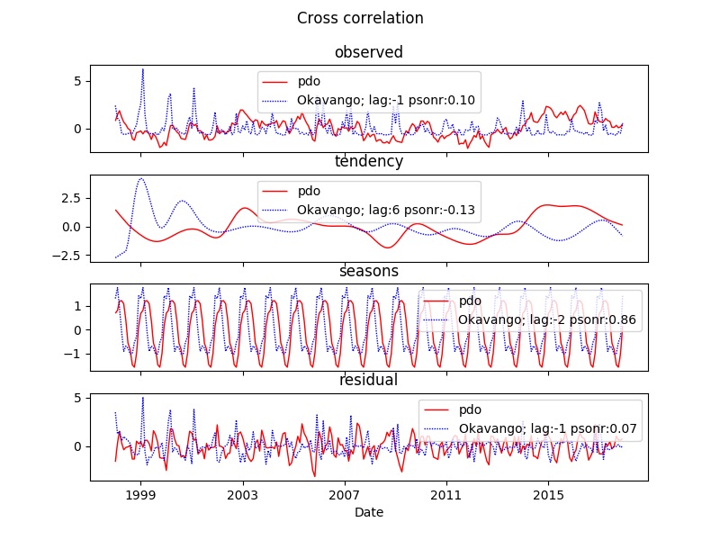
The cross correlation process can decompose the time series on the fly and then analyse the cross correlation for any combination of components (tendency, seasons or residual).

  <process processid = 'indexcompxcrosstsgraphancillary' version = '1.3'>
		<parameters
		title='Cross correlation'
		legend = '0'
		ylabel = ''
		xcrosstendency='True'
		xcrosseason='True'
		xcrossresidual='True'
		></parameters>
		<srcpath volume = "karttur3tb" hdrfiletype = 'tif' datfiletype = 'tif'></srcpath>
		<dstpath volume = "karttur3tb" hdrfiletype = 'tif' datfiletype = 'tif'></dstpath>
		<srccomp>
			<trmm-3b43v7-precip  source = "trmm" product = "3b43" folder = "rainfall" band = "trmm-3b43v7-precip" prefix = "rainfall" suffix = "v7-f">
			</trmm-3b43v7-precip>
		</srccomp>
		<xy id ='Okavango' x='35' y='-22' obscolor = 'b' tendencycolor = 'b'  seasoncolor = 'b' residualcolor = 'b'></xy>
		<index id='pdo' obscolor = 'r' tendencycolor = 'r' seasoncolor = 'r' residualcolor = 'r'></index>
	</process>

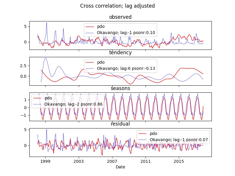
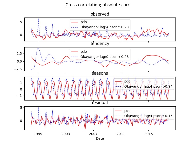
When correlating a single index and a single local observation, setting the parameter lagplot to True infers the identified lag and shifts the plotted time series accordingly. By setting the parameter abs to True the best fitted lag is calculated from the absolute cross correlation. In effect this means that a highly negative (“out of phase”) correlation will be identified if it is stronger than the best positive cross correlation. The figure below shows all four possible combinations of the parameters lagplot and abs for the PDO index and rainfall at the Okavango Delta in Botswana. The differences are easiest to see in the correlations of the seasonal signal.

Cross correlation between the Pacific Decadal Oscillation (PDO) and local rainfall at Okavango (Botswana). The top left panel shows the un-adjusted comparisons and the top right panel the lag adjusted comparisons. The bottom left panel shows the same as the top left but with the best lag calculated from the absolute cross correlation. The bottom right pane shows the lag adjusted time series for the best absolute lag.

Multiple indexes

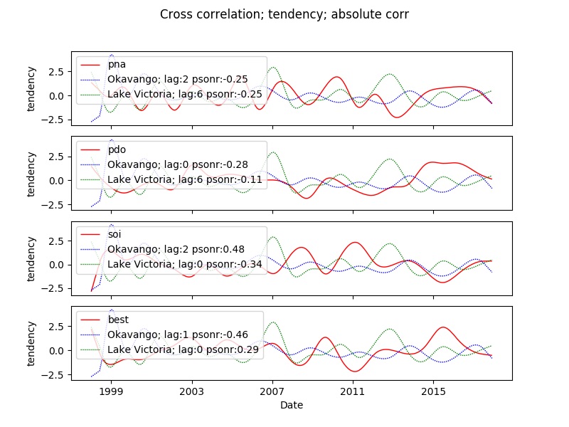
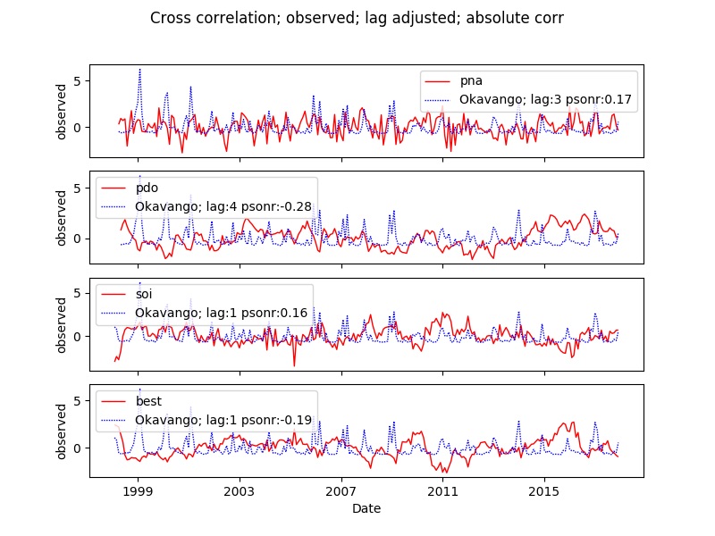
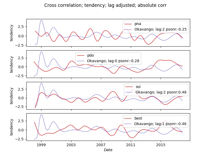
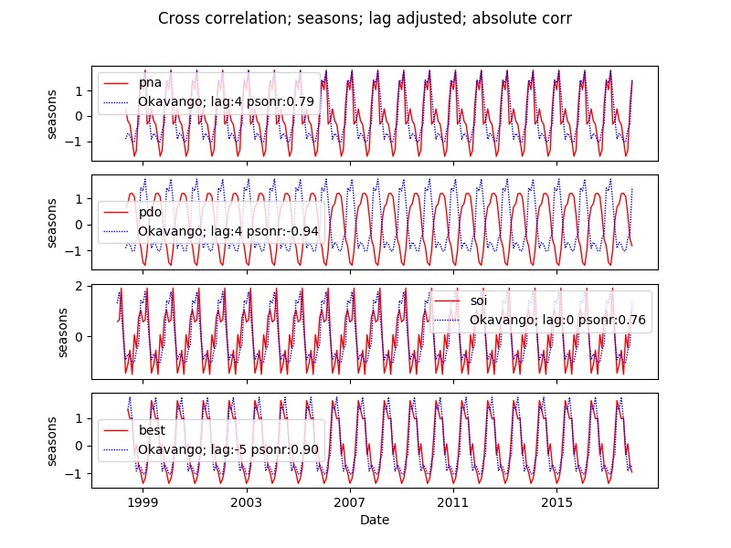
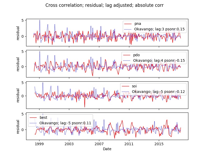
You can compare multiple indexes in the same plot. Each index will be presented as a subplot. Thus you can only compare one kind of time series component (observation, tendency, seasons or residual) when comparing multiple indexes. The example compares several indexes with the rainfall over the Okavango Delta. The example code is for tendency. All examples plot the adjusted lag and all identify the absolute best cross correlation.

  <process processid = 'indexcompxcrosstsgraphancillary' version = '1.3'>
  <parameters
  title='Cross correlation'
  legend = '0'
  ylabel = ''
  lagplot='False'
  abs='True'
  xcrossobserved='False'
  xcrosstendency='True'
  ></parameters>
  <srcpath volume = "karttur3tb" hdrfiletype = 'tif' datfiletype = 'tif'></srcpath>
  <dstpath volume = "karttur3tb" hdrfiletype = 'tif' datfiletype = 'tif'></dstpath>
  <srccomp>
    <trmm-3b43v7-precip  source = "trmm" product = "3b43" folder = "rainfall" band = "trmm-3b43v7-precip" prefix = "rainfall" suffix = "v7-f">
    </trmm-3b43v7-precip>
  </srccomp>
  <xy id ='Okavango' x='35' y='-22' obscolor = 'b' tendencycolor = 'b'  seasoncolor = 'b' residualcolor = 'b'></xy>
  <index id='pna' obscolor = 'r' tendencycolor = 'r' seasoncolor = 'r' residualcolor = 'r'></index>
  <index id='pdo' obscolor = 'r' tendencycolor = 'r' seasoncolor = 'r' residualcolor = 'r'></index>
  <index id='soi' obscolor = 'r' tendencycolor = 'r' seasoncolor = 'r' residualcolor = 'r'></index>
  <index id='best' obscolor = 'r' tendencycolor = 'r' seasoncolor = 'r' residualcolor = 'r'></index>
  </process>

Cross correlations between climate indexes (pna, pdo, soi, best) and local rainfall at Okavango (Botswana). The panels show different components after time series decompostion of both series. All time series have the best fitted abosulte lag adjusted to fit the two time series.

You can plot multiple indexes together with multiple sites, but still with only one time series component and with the parameter lagplot set to False (= default).

Cross correlation between different climate indexes and local rainfall at Okavango (Botswana) and Lake Victoria (Uganda).