Introduction

A time series can be thought of as a combination of an average level, seasonal effects, long term tendencies and random noise. Time series decomposition aims at identifying these four (4) components:

level: the long term average
seasonality: short-term repeating patterns
trend: Increasing or decreasing tendencies
noise: random variations

Additive and multiplicative components

Time series tend to be of two different kinds, additive or multiplicative. In additive models the trend (or tendency) over time, if any, tends to be linear and the components are added together:

value = level + seasonality + trend + noise

Multiplicative models show non-linear tendencies over time, where the tendency can be negative or positive and for instance described using exponential or quadratic functions. Multiplicative models do not accept any negative values and are not suitable for decomposition of for example climate indexes. In multiplicative models the components are multiplied together:

value = level * seasonality * trend * noise

Prerequisites

You must have setup Karttur’s GeoImagine Framework as described in earlier posts. You must also have added the climate indexes and atmospheric carbon dioxide (CO₂) records to the database.

If you want to use the ore advanced decomposition method you must also install the package seasonal.

The plotting functions of Karttur’s GeoImagine Framework make use of matplotlib.

Framework process

In this post you will use the climate indexes and the Mauna Loa record of atmospheric CO2 introduced in the previous posts.

Karttur’s GeoImagine Framework includes two different methods for time series decomposition; a classical, or naive, decomposition as available in the statsmodel package, and a more advanced method from a customized version of the seasonal package.

The combined time series decomposition and plotting function for climate indexes (and other database recorded) time series in Karttur’s GeoImagine Framework is componentdbtsgraphancillary.

Additive decomposition

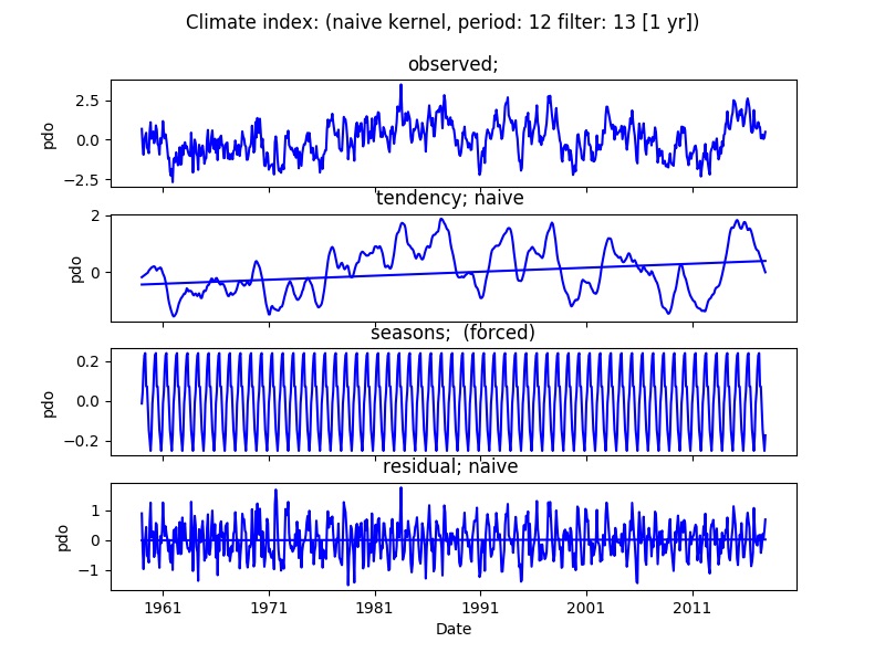
By default the componentdbtsgraphancillary applies an additive model and the more advanced decomposition from the modified seasonal package. To use the naive (classical) decomposition set the parameter naive to True. The example below performs a naive, additive decomposition of a single climate index (pdo = Pacific Decadal Oscillation).

<?xml version='1.0' encoding='utf-8'?>
<plotdbtsclimate>
<process processid = 'componentdbtsgraphancillary' version = '1.3'>
		<parameters
		ylabel='pdo'
		title='Climate index'
		naive='True'
		></parameters>
		<index id ='pdo' obsformat = 'b-' tendencyformat = 'b-' regressformat = 'b-' seasonformat = 'b-' residualformat = 'b-'></index>
</process>
</plotdbtsclimate>

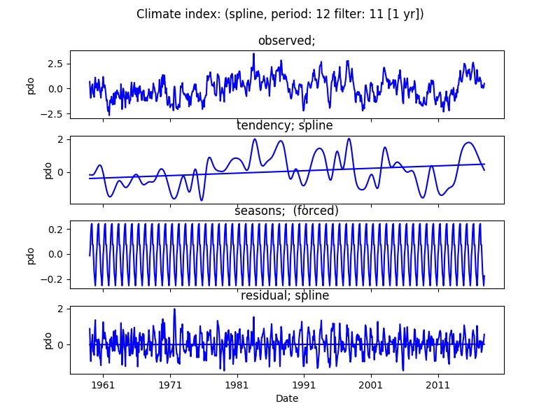
To change to a more advanced additive model, just remove the parameter naive, or set it to False (parameter default value). The figure below compares the decomposition results for both methods.

Decomposed time series of the Pacific Decadal Oscillation (PDO) climate index. The left image shows a classic or naive model and the right a spline based model.

Multiplicative decomposition

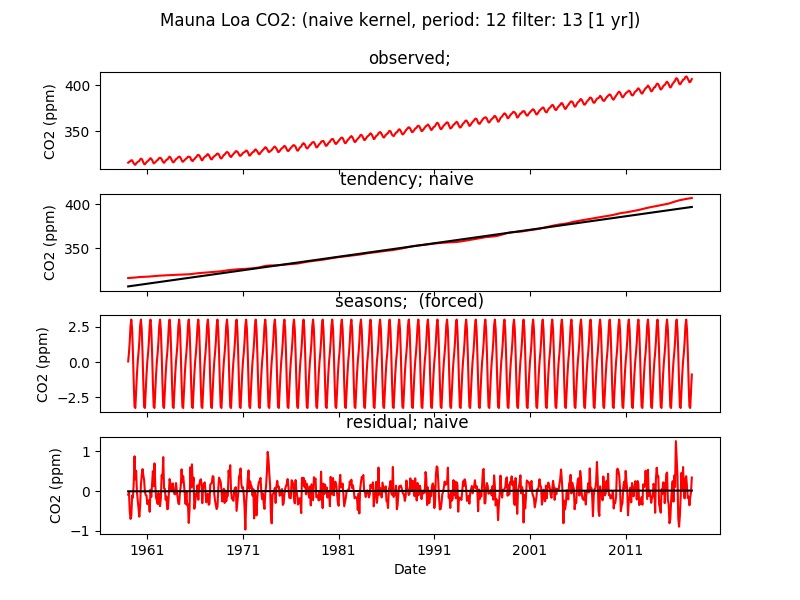
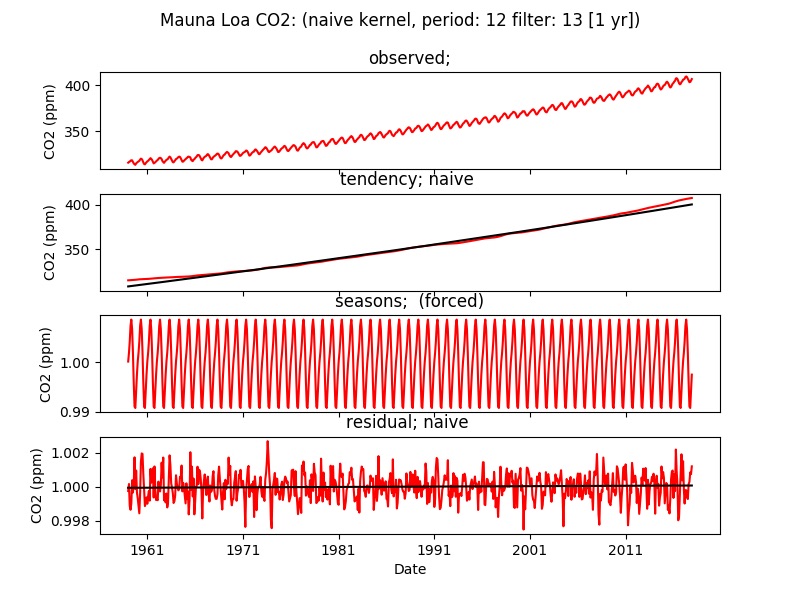
The time series of atmospheric CO2 content at Mauna Loa, Hawaii, show a non-linear increase from 1958 to 2017. The xml file below shows how to generate a mutiplicative naive decomposition using Karttur’s GeoImagine Framework. The multiplicative model is only implemented for the naive (classical) decomposition. The regression model for capturing the tendency for mulitplicative models is simply using the log-normal transformation and then applies a robust liner regression model (Theil-Sen).

Other alternatives include using numpy.polyfit or scipy.optimize.curve_fit, but that is not implemented at present.

The xml file for running a naive, multiplicative decomposition using the monthly Mauna Loa data:

<?xml version='1.0' encoding='utf-8'?>
<plotdbtsclimate>
	<userproj userid = 'karttur' projectid = 'karttur' tractid= 'karttur-trmm' siteid = '*' plotid = '*' system = 'ancillary'></userproj>
	<period startyear = "1959" startmonth='01' endyear = "2017" endmonth='12' timestep='M'></period>
	<process processid = 'componentdbtsgraphancillary' version = '1.3'>
		<parameters
		ylabel='CO2 (ppm)'
		title='Mauna Loa CO2'
		naive='True'
		additive='False'
		></parameters>
		<index id ='co2-mm-mlo' obsformat = 'r-' tendencyformat = 'r-' regressformat = 'k-' seasonformat = 'r-' residualformat = 'r-'></index>
	</process>
</plotdbtsclimate>

To change to an additive model, just remove the parameter additive or change to additive=’True’ (as this is the default it does not matter if you state it explicitly or not).

Decomposed time series of atmospheric CO2 from Mauna Loa, Hawaii. The left image shows an additive model and the right a multiplicative model.

Resources

How to Decompose Time Series Data into Trend and Seasonality by Jason Brownlee at Machine Learning Mastery.