
Contents - Introduction - Prerequisites - Python module skeleton - Model setup - Model parameterizations - Dataset preparation - Plot function - Train/test model approach - Models - Linear models - Ordinary Least Square (OLS) regression - Theil-Sen regression - Add other linear regressors - Non-linear models - k-nearest neighbors regression - Decision Tree Regression - Random Forest Regression - Support Vector Machine regression - Cross validation approach - Resources
Introduction
In the previous post we built a Python module (.py) file in Eclipse for machine learning using linear regression. In this post you will look at other algorithms for machine learning and predicting continuous phenomena using regressions. If instead you are looking for predicting crisp classes from continuous co-variates, Jason Brownlee’s post on Spot-Check Regression Machine Learning Algorithms in Python with scikit-learn is the place to start.
You can copy and paste the code in the post, but you might have to edit some parts: indentations does not always line up, quotations marks can be of different kinds and are not always correct when published/printed as html text, and the same also happens with underscores and slashes.
The complete code is also available here.
Prerequisites
This post is a continuation of the post on Introduction to machine learning, and the prerequisites are the same: a Python environment with numpy, pandas, sklearn (Scikit learn) and matplotlib installed.
Python module skeleton
We are going to start with a similar Python module skeleton and dataset import function as in the previous post. If you are not familiar with the Python code below, you can build the skeleton step by step by following the previous post, otherwise just copy and paste the code below to an empty Python module (.py file). The skeleton is set up for using the dataset on Boston house prices introduced in the previous post.
import numpy as np
import pandas as pd
from sklearn import model_selection
from sklearn import linear_model
from sklearn.neighbors import KNeighborsRegressor
from sklearn.tree import DecisionTreeRegressor
from sklearn.ensemble import RandomForestRegressor
from sklearn.svm import SVR
from sklearn.metrics import mean_squared_error, r2_score

class RegressionModels:
    '''Machinelearning using regression models
    '''
    def __init__(self, columns,target):
        '''creates an instance of RegressionModels
        '''
        self.columns = columns
        self.target = target

    def ImportUrlDataset(self,url):
        self.dataframe = pd.read_csv(url, delim_whitespace=True, names=self.columns)

    def ExtractDf(self,omitL):
        #extract the target column as y
        self.y = self.dataframe[self.target]
        #appeld the target to the list of features to be omitted
        omitL.append(self.target)
        #define the list of data to use
        self.columnsX = [item for item in self.dataframe.columns if item not in omitL]
        #extract the data columns as X
        self.X = self.dataframe[self.columnsX]

if __name__ == ('__main__'):
    columns = ['CRIM', 'ZN', 'INDUS', 'CHAS', 'NOX', 'RM', 'AGE', 'DIS', 'RAD', 'TAX', 'PTRATIO', 'B', 'LSTAT', 'MEDV']
    target = 'MEDV'
    regmods = RegressionModels(target)
    regmods.ImportUrlDataset('https://archive.ics.uci.edu/ml/machine-learning-databases/housing/housing.data')
Model setup
To test the predictive power of different models, we need a functions for doing the testing. There will be two different alternative model testings, one dividing the dataset in training and test subsets, and one using cross validation iterations. Both can use the same models, and we need a common function for model selection and parameterization.
Model parameterizations
You are going to use an ensemble of different models for testing and evaluating their predictive powers. All models can be defined using different sets of parameters, and to allow any user defined parameterizations we will use dictionaries. If you are not familiar with Python dictionaries, they have a keyword (key) and then values associated with the key. A dictionary can also contain another dictionary, and you are going to use that approach here for defining which models to test and their parameter setting. In the code below, the variable modD is the dictionary. The ModelSelectSet below must be part fo the class RegressionModels in the skeleton.
    def ModelSelectSet(self,modD):
        self.models = []
        if 'OLS' in modD:
            self.models.append(('OLS', linear_model.LinearRegression(**modD['OLS'])))
        if 'TheilSen' in modD:
            self.models.append(('TheilSen', linear_model.TheilSenRegressor(**modD['TheilSen'])))
        if 'KnnRegr' in modD:
            self.models.append(('KnnRegr', KNeighborsRegressor(**modD['KnnRegr'])))
        if 'DecTreeRegr' in modD:
            self.models.append(('DecTreeRegr', DecisionTreeRegressor(**modD['DecTreeRegr'])))
        if 'SVR' in modD:
            self.models.append(('SVR', SVR(**modD['SVR'])))
        if 'RandForRegr' in modD:
            self.models.append(('RandForRegr', RandomForestRegressor(**modD['RandForRegr'])))
The code snippet below shows the principle for constructing the modD dictionary (the example is for an ordinary linear regression model with no special parameterizations).
    modD = {}
    modD['OLS'] = {}
But before testing any models you must create some more functions.
Dataset preparation
First you need to prepare the dataset by defining which variables (columns in the dataset) to use as independent and dependent variables, and then also add the plot function that will show the graphical results.
In the skeleton that you created in the beginning, the function for extracting the variables to use as dependent and independent variables, is already defined (ExtractDf). Call it after you retrieved the dataset in the __main__ section. You have to give the target variable to predict (‘MEDV’) and then you can exclude other variables in your dataaset by listing them inside the squared brackets. In this post you will use all other variables for predicitng ‘MEDV’ (median housing prices).
regmods.ExtractDf('MEDV', [])
Plot function
Then also add the function for plotting the model predictions, which is an identical copy of the function defined in the previous post
def PlotRegr(self, obs, pred, title, color='black'):
    pyplot.xticks(())
    pyplot.yticks(())
    fig, ax = pyplot.subplots()
    ax.scatter(obs, pred, edgecolors=(0, 0, 0),  color=color)
    ax.plot([obs.min(), obs.max()], [obs.min(), obs.max()], 'k--', lw=3)
    ax.set_xlabel('Observations')
    ax.set_ylabel('Predictions')
    pyplot.title(title)
    pyplot.show()
Train/test model approach
The first model test bed (RegrModTrainTest) will divide the dataset into subsets for training and testing. By default the latter will be 30 % (0.3), and the former 70 %. We use a larger fraction for calibrating the model to avoid underfitting, but not too large to avoid overfitting (mush less likely to happen). You can change that when calling the function, as described in the previuos post. By default the graphical plot of the model prediction for the test subset will be shown.
    def RegrModTrainTest(self, testsize=0.3, plot=True):
        #Split the data into training and test substes
        X_train, X_test, y_train, y_test = model_selection.train_test_split(self.X, self.y, test_size=testsize)
        #Loop over the defined models
        for m in self.models:
            #Retrieve the model name and the model itself
            name,mod = m
            #Fit the model
            mod.fit(X_train, y_train)
            #Predict the independent variable in the test subset
            predict = mod.predict(X_test)
            #Print out the model name
            print 'Model: %s' %(name)
            #Print out RMSE
            print("    Mean squared error: %.2f" \
                % mean_squared_error(y_test, predict))
            #Print explained variance score: 1 is perfect prediction
            print('    Variance score: %.2f' \
                % r2_score(y_test, predict))
            if plot:
                title = ('Model: %(mod)s; RMSE: %(rmse)2f; r2: %(r2)2f' \
                          % {'mod':name,'rmse':mean_squared_error(y_test, predict),'r2': r2_score(y_test, predict)} )
                self.PlotRegr(y_test, predict, title, color='green')
Models
In the previous post we used linear regression for predicting housing prices in Boston. In this post you will try some more linear models, and then some other non-liner models. But let us start with some linear models.
Linear models
Linear regression models assume that the independent variables are normally distributed, and preferable unrelated to each other. In some cases your model predictions might be biased due to skewness or outliers, and you want a more robust estimator. There are a suite of linear models available in the Scikit learn (sklearn) package to choose from to bypass some of the shortcomings with an ordinary least square (OLS) regression. To understand the differences between the models and select one that suites your problem you can look at the Scikit learn page on Generalized Linear Models. You can easily add any model you want to test to the python module (will be explained below).
Ordinary Least Square (OLS) regression
The OLS regression is the classical regression model, in sklearn it is called LinearRegression. To use it in our testbed, add the following lines to the end of the __main__ section of the Python module:
    modD = {}
    modD['OLS'] = {}
    regmods.ModelSelectSet(modD)
    regmods.RegrModTrainTest()
If you run the Python module, you should get the results from the OLS regression both as text, and as a graphical plot. If it does not work, you can copy and paste the entire module code thus far from under the “Hide/show” button.
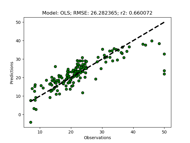
If you test the OLS regressor, your model results will most likely vary slightly compared to the results in the plot above. That is because the splitting of the dataset into training and test subsets is random.
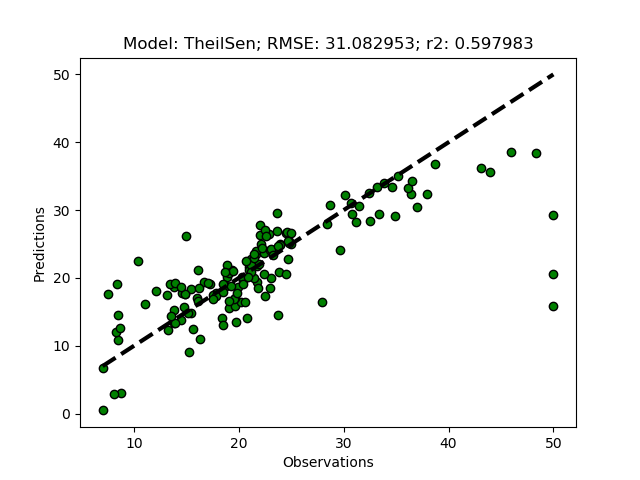
Theil-Sen regression
The Theil-Sen regression was developed for achieving a more robust model, by identifying the median slope for subsets of the complete dataset. You can define the number of susbsets (parameter: n_subsamples). If not given, sklearn will seek the most robust solution automatically. The Theil-Sen regression is commonly used for estimating change in for example climate data over time. To use the Theil-Sen regressor in our testbed, just add it in the __main__ section before you call ModelSelectSet (if you do not want to redo the OLS, put a “#” sign to comment it out):
    modD = {}
    #modD['OLS'] = {}
    modD['TheilSen'] = {}
    regmods.ModelSelectSet(modD)
    regmods.RegrModTrainTest()
To run the Theil-Sen regression with a predefined number of subsets, set n_subsamples as a parameter+value pair in modD:
modD['TheilSen'] = {'n_subsamples':10}
Add other linear regressors
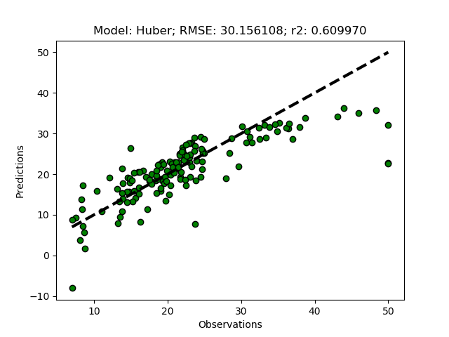
To add other linear regressors you only need to add two lines. First you have to invent a name or abbreviation, then add the regressor in the ModelSelectSet function with the chosen name, and then add the name (and any parameter you want to set) to the modD dictionary in the __main__ section. To try it out, add the Huber regression model as ‘Huber’. First add Huber to the ModelSelectSet function.
        if 'Huber' in modD:
            self.models.append(('Huber', linear_model.HuberRegressor(**modD['Huber'])))
And then add ‘Huber’ in the modD dictionary.
modD['Huber'] = {'epsilon':1.25}
If you run the python module, you should get the results also for the Huber regressor (with the parameter epsilon set to a lower number the result is less sensitive to outliers, 1.35 is the default). The Huber regression sets lower weights to outliers, and thus also generates a more robust model, but using other principles compared to the Theil-Sen regression.
Non-linear models
Scikit learn (sklearn) also contains other type of models than generalized linear models. To apply these models is no different compared to applying linear models. Also the non-linear models can be used without parameterizations, but to get good results it is often required to adjust the parameters to fit the dataset that is modelled.
The different kinds of non-linear regression models (predicting continuous variables) to be tested in this post include:
The non-linear methods included below are already imported in the module skeleton. All you need to do to test the models is to add the method you want to try to the modD dictionary.
k-nearest neighbors regression
The k-nearest neighbors regressor predicts the independent (target) variable from the local (rather than global) neighborhood. To test the model, just add it as ‘KnnRegr’ to the modD dictionary in the __main__ section.
modD['KnnRegr'] = {}
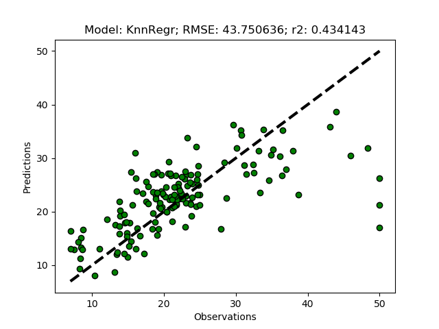
The default number of neighbors (n_neighbors) is 5, to increase to 8, add the parameter+value pair to the dictionary.
modD['KnnRegr'] = {'n_neighbors':8}
There are several more parameters that you can set, all outlined in the Scikit learn page for KNeighborsRegressor
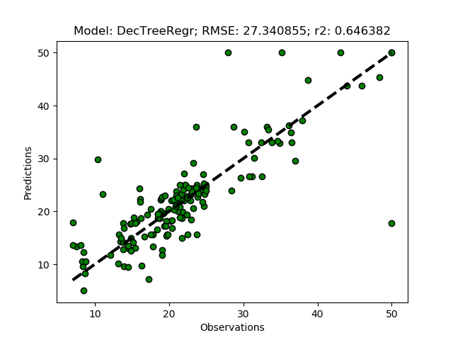
Decision Tree Regression
A decision tree regressor uses some measures of fit (for example mean square error) to split the data iteratively and hierarchically in order to create a prediction. Try the sklearn DecisionTreeRegressor by adding ‘DecTreeRegr’ to the modD dictionary and run the python module.
modD['DecTreeRegr'] = {}
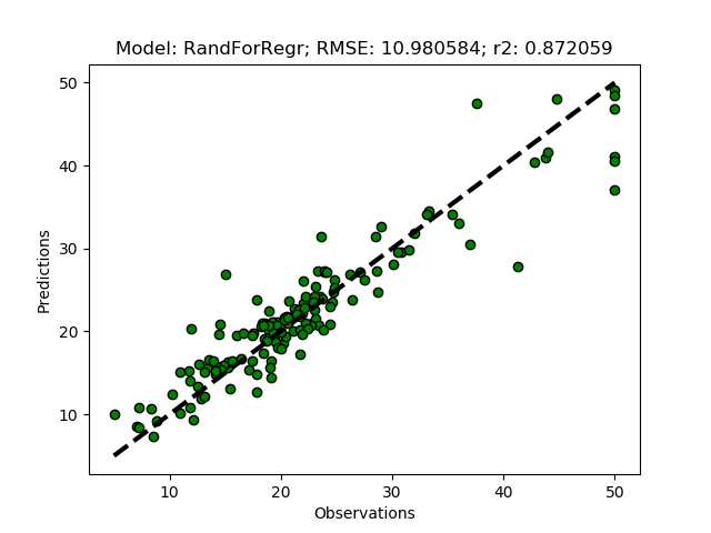
Random Forest Regression
The Random Forest Regressor is a meta (or ensemble) regression method, that uses elements from other methods in combination. It should thus give better predictions compared to the previous methods. To try it out add it as ‘RandForRegr’ to the modD dictionary.
modD['RandForRegr'] = {}
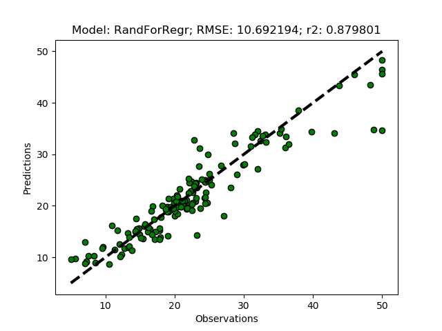
To improve the prediction further you can increase the number of trees in the forest (n_estimators) from the default (10) to 30 or more.
modD['RandForRegr'] = {'n_estimators': 30}
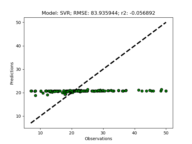
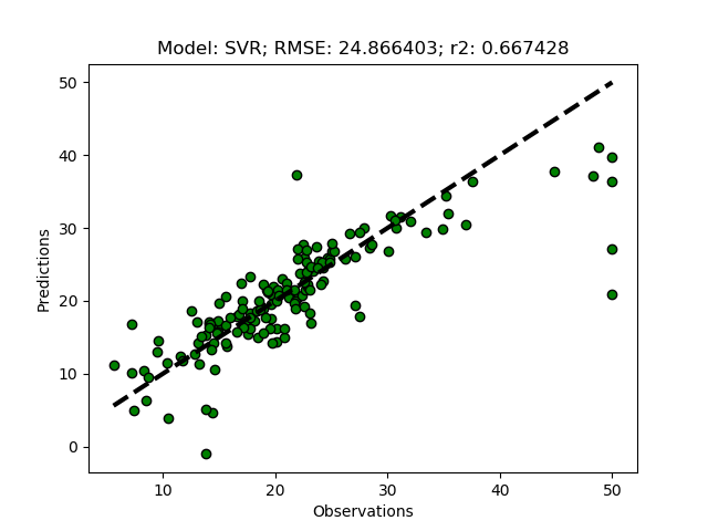
Support Vector Machine regression
The support vector machine regressor (SVR) usually requires a more careful parameterization. First try it it out using the default settings by adding ‘SVR’ to the modD dictionary.
modD['SVR'] = {}
If you run the SVR model without any parameterizations, you should get a flat prediction. The default kernel (a small matrix identifying local variations) Radial Basis Function (‘rbf’) fits the local data too well, and in combination with the default punishment parameter (C) for non-fitted records, and the default threshold parameter (epsilon) for accepting variations in the kernel, the regression does not predict the independent variable. You need to set the parameters for kernel, C and/or epsilon.
modD['SVR'] = {'kernel':'linear','C':1.5,'epsilon':0.05}
Cross validation approach
Above you tested various models by dividing the dataset into training and test subsets. It is often better to use an iterative cross validation wile leaving out different subsets of the data in each iteration (see previous post). To implement that for testing the models defined in the python module that you built in this post, you just need to a new function (RegrModKFold).
  def RegrModKFold(self,folds=10, plot=True):
        # set the kfold
        kfold = model_selection.KFold(n_splits=folds)
        for m in self.models:
            #Retrieve the model name and the model itself
            name,mod = m
            # cross_val_predict returns an array of the same size as `y` where each entry
            # is a prediction obtained by cross validation:
            predict = model_selection.cross_val_predict(mod, self.X, self.y, cv=kfold)
            # to retriece regressions scores, use cross_val_score
            scoring = 'r2'
            r2 = model_selection.cross_val_score(mod, self.X, self.y, cv=kfold, scoring=scoring)
            # The correlation coefficient
            #Print out the model name
            print 'Model: %s' %(name)
            #Print out correlation coefficients
            print('    Regression coefficients: \n', r2)
            #Print out RMSE
            print("Mean squared error: %.2f" \
                  % mean_squared_error(self.y, predict))
            #Explained variance score: 1 is perfect prediction
            print('Variance score: %.2f' \
                % r2_score(self.y, predict))

            if plot:
                title = ('Model: %(mod)s; RMSE: %(rmse)2f; r2: %(r2)2f' \
                          % {'mod':name,'rmse':mean_squared_error(self.y, predict),'r2': r2_score(self.y, predict)} )
                self.PlotRegr(self.y, predict, title, color='blue')
And then comment out the function RegrModTrainTest and add the new function RegrModKFold in the __main__ section.
    #regmods.RegrModTrainTest()
    regmods.RegrModKFold()
The complete module is hidden under the button below, and available at GitHub.
Resources
Spot-Check Regression Machine Learning Algorithms in Python with scikit-learn by Jason Brownlee
Train/Test Split and Cross Validation in Python by Adi Bronshtein
Completed python module on GitHub.