
Contents - Introduction - Prerequisites - Machinelearning for mapping - Python environment setup - Get dataset - Get the dataset from sklearn - Get the dataset from the internet - Data exploration - Plot the data - Dependent and independent variables - Ordinary regression - Regression model - Cross validation iterators - Resources
Introduction
When I use Python for machinelearning I tend to use the machinelearning package as a reference, and then I read the excellent posts on machinelearningmastery.com written by Jason Brownlee to get more flesh on the bones. If you are looking for a more general introduction to applied machinelearning with Python, I would recommend Your First Machine Learning Project in Python Step-By-Step by Jason Brownlee. This post is more of an introduction on how to create a python module for regression modelling in machinelearning.
You can copy and paste the code in the post, but you might have to edit some parts: indentations does not always line up, quotations marks can be of different kinds and are not always correct when published/printed as html text, and the same also happens with underscores and slashes.
The complete code is also available here.
Prerequisites
To follow this post you need to have a Python environment with numpy, Pandas and sklearn (Scikit learn) installed. The most convenient way to get these Python packages is to install Anaconda. To write and test the code, an Integrated Development Environment (IDE) like Eclipse is the best alternative. Other posts in this blog describe how to install Anaconda and how to Install Eclipse for Python Development using Anaconda. The rest of this post will assume that you have all the Python packages installed, and an IDE for writing the code.
Python environment setup
Start Eclipse (or another IDE with a python interpreter) and either create a new PyDev project with a new PyDev Package, or create a PyDev package within an existing project. The create a PyDev module (.py file). Copy and paste the package imports below to the top of the PyDev module.
#numpy: for handling 2d (array) data
import numpy as np
#Pandas: for reading and organizing the data
import Pandas as pd
#Scikit learn (sklearn) machinelarning package (selected sub-packges and modules)
from sklearn import model_selection
from sklearn.linear_model import LinearRegression
from sklearn.metrics import mean_squared_error, r2_score
Below the imports, create a new class called RegressionModel. It will be initiated by giving the columns (features) and the target (dependent variable) of the dataset you are going to model.
class RegressionModel:
    '''Machinelearning using linear regression
    '''
    def __init__(self,columns,target):
        '''creates an empty instance of RegressionMode
        '''
        self.columns = columns
        self.target = target
Also create the __main__ section of your module, at the very bottom of the .py file. In the __main__ section, create an instance of the class RegressionModel by calling it. As you do not yet know the columns or target of the dataset you are going to use, just give an empty list (with no columns) and an empty name. In the example below, the instance of the class RegressionModel is called “regmod”.
if __name__ == ('__main__'):
    columns = list()
    target = ''
    #A list can also be initiated like this: columns = []
    regmod = RegressionModel(columns,target)
You now have a skeleton python module, and the next thing you need is an import function to get the dataset to model using machinelearning.
Get dataset
You need a dataset with continuous variables (rather than classes), and in this post we will use a standard machinelearning dataset on housing prices in Boston. There are different ways to capture the dataset, and you can try all, or select one.
Get the dataset from sklearn
As the housing dataset is used in the official manuals of Scikit learn, it is available as a module in sklearn. To get it, just import the sklearn package for datasets, and then you have access to the dataset. If you use this route, you have to create the Pandas dataframe object that you are going to use for plotting the data after importing the dataset. The function below imports the housing dataset, and creates a Pandas dataframe. Copy and paste the function as part of the class RegressionModel.
    def ImportSklearnDataset(self):
        #the Scikit (sklearn) package includes some datasets
        from sklearn import datasets
        #Load the Boston dataset from the datasets package library
        dataset = datasets.load_boston()
        #The sklearn organised dataset divides the dataset between the independent variables ("data") and the dependent variable ("target").
        #To create a Pandas dataframe you have to stack them when creating the Pandas dataframe
        self.dataframe =  pd.DataFrame(data=np.column_stack((dataset.data,dataset.target)), columns=self.columns)
Get the dataset from the internet
You can also load the data directly from the internet by using Pandas and the url to the dataset. The function is more generic and can be used also to import other datasets, but you must give the url link when calling the function. Also this function should be part of the class RegressionModel.
    def ImportUrlDataset(self,url):
        self.dataframe = pd.read_csv(url, delim_whitespace=True, names=self.columns)
Downloading the dataset
You can also download the dataset, and use the function above (ImportUrlDataset) but instead of the url just give the local path on your machine to where you saved the downloaded dataset.
On the download page you also find the document “housing.names”, that lists the names as given in the variable columns in the code, and what they mean (for example: MEDV = median value).
Calling your import function
If you looked at the download site for the housing data, you would have seen the column names or headers. You can now complete the __main__ section, and call one of the import alternatives.
if __name__ == ('__main__'):
    columns = ['CRIM', 'ZN', 'INDUS', 'CHAS', 'NOX', 'RM', 'AGE', 'DIS', 'RAD', 'TAX', 'PTRATIO', 'B', 'LSTAT', 'MEDV']
    target = 'MEDV'
    regmod = RegressionModel(columns, target)
    #either
    regmod.ImportSklearnDataset()
    #or
    regmod.ImportUrlDataset('https://archive.ics.uci.edu/ml/machine-learning-databases/housing/housing.data')
To see the complete code so far, click the button.
Data exploration
Create a function as part of the class RegressionModel for exploring the dataset:
    def Explore(self, shape=True, head=True, descript=True):
        if shape:
            print(self.dataframe.shape)
        if head:
            print(self.dataframe.head(12))
        if descript:
            print (self.dataframe.describe())
When calling the function Explore, by default it will show shape, head and description (shape=True, head=True, descript=True). Call the function by adding the following line at the bottom of __main__ section:
regmod.Explore()
If you only want to see the description, use the following call instead:
regmod.Explore(False, False, True)
Plot the data
To plot the data, you need to install the package matplotlib:
from matplotlib import pyplot
I never got pyplot to work with this, supposedly correct, installation. In my present IDE on a macOS (10.13.2) I have to do it like this instead:
import matplotlib
matplotlib.use(\'TkAgg\')
from matplotlib import pyplot
Because we are going to use matplotlib also in other functions, the import should be at the top of the module, with the other imports.
To keep the code a bit tidy, create another function (PlotExplore) for plotting the dataframes. Again it should be a function within the class RegressionModel.
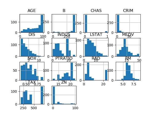
def PlotExplore(self, histo = True, box = True):
from math import sqrt,ceil
if histo:
self.dataframe.hist()
pyplot.show()
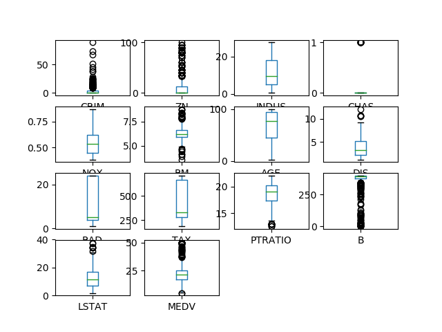
if box:
nrows = int(round(sqrt(len(self.dataframe.columns))))
ncols = int(ceil(len(self.dataframe.columns)/float(nrows)))
self.dataframe.Plot(kind='box', subplots=True, layout=(ncols,nrows))
pyplot.show()
Call the PlotExplore function from the __main__ section:
regmod.PlotExplore()
The function calculates the rows (nrows) and columns (ncols) for displaying box-whisker (box) subplots. By default the function will show both the histograms and the the box-whisker plots, but you can set that when calling the function as explained above. To show only the box-whisker plot, change the call accordingly.
regmod.PlotExplore(False, True)
Dependent and independent variables
If you retrieved the housing dataset from the sklearn library, it was already divided between independent variables and the dependent variable (MEDV in this dataset). If you imported the data from the internet, or as a local file, all the data came as a single matrix. When you created the Pandas dataframe, you linked each feature to a column with a name.
To use sklearn for modelling, you must tell sklearn which data represent the dependent and independent features. This can be done in different ways, but you will create a generic function (ExtractDf) that will create two numpy matrices, one for the independent (co-variates) and one for the dependent (target) variables. Following the standard syntax of sklearn examples, we will call the former X and the latter y.
    def ExtractDf(self,target,omitL = []):
        #extract the target column as y
        self.y = self.dataframe[target]
        #append the target to the list of features to be omitted
        omitL.append(target)
        #define the list of data to use
        self.columnsX = [item for item in self.dataframe.columns if item not in omitL]
        #extract the data columns as X
        self.X = self.dataframe[self.columnsX]
The function ExtractDf extracts the target column, and then you can additionally add a list of other features that are included in the dataframe, but that you do not want to use in the modeling. To extract the target (y) and the co-variates (X) add the following lines to the end of the __main__ section. The three print statements are just for confirming that the extraction went OK. You can skip, or delete, them after confirming that it worked as expected.
    target ='MEDV'
    omitL =[]
    regmod.ExtractDf(omitL)
    print (regmod.dataframe.shape)
    print (regmod.y.shape)
    print (regmod.X.shape)
If you run the python module, you should get the shapes of the original dataframe, the target (y) data, and the independent (X) co-variates.
(506, 14)
(506,)
(506, 13)
If it does not work, you can get the code written thus far by clicking the button below.
Ordinary regression
The Scikit learn (sklearn) package can be used for ordinary regressions (without making use of the modelling capabilities). To run a multiple regression using all the data, copy and the paste the MultiRegression and PlotRegr functions.
def PlotRegr(self, obs, pred, title, color='black'):
pyplot.xticks(())
pyplot.yticks(())
fig, ax = pyplot.subplots()
ax.scatter(obs, pred, edgecolors=(0, 0, 0), color=color)
ax.plot([obs.min(), obs.max()], [obs.min(), obs.max()], 'k--', lw=3)
ax.set_xlabel('Observations')
ax.set_ylabel('Predictions')
pyplot.title(title)
pyplot.show()
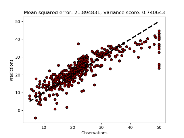
def MultiRegression(self, plot=True):
regr = LinearRegression()
#Fit the regression to all the data
regr.fit(self.X, self.y)
#Predict the independent variable
predict = regr.predict(self.X)
#The coefficients
print('Coefficients: \n', regr.coef_)
#The mean squared error
print("Mean squared error: %.2f" \
% mean_squared_error(self.y, predict))
#Explained variance score: 1 is perfect prediction
print('Variance score: %.2f' \
% r2_score(self.y, predict))
if plot:
title = ('Mean squared error: %(rmse)2f; Variance score: %(r2)2f' \
% {'rmse':mean_squared_error(self.y, predict),'r2': r2_score(self.y, predict)} )
self.PlotRegr(self.y, predict, title, color='maroon')
The regression above takes all the data and fits a model, then predicts the independent variable (y) from the regression. This is a naive approach, and does not perform any independent calibration and validation. It the variable plot is set to True, the function assembles a title, and calls PlotRegr. Calling PlotRegr requires the observed and predicted numpy arrays, and the title; additionally a color can be defined. If no color is given the scatter plot of each pair observed-predicted is defaulted to black. In the example above it is given as maroon. The plot function is called from within MultiRegression. To test the regression you only need to add a single line at the end of the __main__ section.
regmod.MultiRegression()
Regression model
To create a calibrated and validated model, you must divide the dataset into 2 parts, one (larger) chunk used for model calibration and one smaller to use for model validation. To avoid both overfitting and underfitting the latter should contain about 20 to 40 % of the data. Scikit learn contains a function that splits the data for you, just add it to your imports at the top of the module:
from sklearn.model_selection import train_test_split
To split the dataset just call the function to split your X (independent data) and y (dependent) datasets:
X_train, X_test, y_train, y_test = train_test_split(self.X, self.y, test_size=testsize)
where testsize is the fraction of the dataset to use for testing (validating) the model (it should then be between approximately 0.2 and 0.4). You need to update the code to use the training datasets (X_train and y_train) for calibrating (training) your regression, and then predict the results using the test datasets (X_test and y_test). You then also need to change the reporting of the results and the plot. The function below have all the necessary changes:
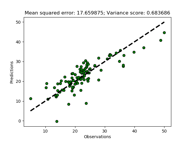
    def MultiRegressionModel(self,testsize=0.3, plot=True):
        #Split the dataset into training and test
        X_train, X_test, y_train, y_test = train_test_split(self.X, self.y, test_size=testsize)
        regr = LinearRegression()
        #Fit the regression to the training data
        regr.fit(X_train, y_train)
        #Predict the independent variable
        predict = regr.predict(X_test)
        #The coefficients
        print('Coefficients: \n', regr.coef_)
        #The mean squared error
        print("Mean squared error: %.2f" \
            % mean_squared_error(y_test, predict))
        #Explained variance score: 1 is perfect prediction
        print('Variance score: %.2f' \
            % r2_score(y_test, predict))
        if plot:
            title = ('Mean squared error: %(rmse)2f; Variance score: %(r2)2f' \
                      % {'rmse':mean_squared_error(y_test, predict),'r2': r2_score(y_test, predict)} )
            self.PlotRegr(y_test, predict, title, color='green')
Instead of hardcoding the fraction of the data that is going to be used for testing the accuracy, I chose to set it as a variable (testsize) with a default value of 0.3. To call the function with another testsize, add that when calling the function; you can also turn off the default plot, by adding False.
regmod.MultiRegressionModel(0.2, False)
Cross validation iterators
The Regression model in the previous section is sensitive to drifts or biases in data. For example, if you sample house prices over time, the prices might drift upwards or downwards unrelated to your features (e.g. by inflation or deflation). Or perhaps the data was sampled from north to south, and for reasons outside the co-variates (another name for the independent data features) the prices are increasing in one of the directions. Under such circumstances it is not good to just split the dataset in two parts. You could solve that by a random split (as Scikit learn does), but you might still be at risk of selecting a training dataset that statistically differs from the test dataset. The way to solve that, and improve your machine learning model, is to iteratively split your dataset and cross validate. In the jargon of machine learning this is called folding. It is easy enough to implement in Scikit learn with the functions KFold and cross_val_predict, both in the package model_selection that you already imported at the beginning.
In the function KFold , you set the number of folds (iterations) as n_splits
kfold = model_selection.KFold(n_splits=10)
You can set other parameters as well, as explained in the Scikit kfold page
To use an iterative model calibration/prediction using kFold, you call the function:
predict = model_selection.cross_val_predict(model, X, y, cv=kfold)
The cross_val_score function has many optional parameters, all given on Scikit cross_val_predict page.
The function cross_val_predict splits the dataset in each fold, so no need to the split the dataset into training and test subsets as in the previous section.
The function cross_val_predict only returns the predictions. To get the scores for each fold, you have to use cross_val_score, and state what score you want to retrieve. To get the scores for the prediction compared to the independent feature to estimate (y) you calculate them by using individual score functions from the sklearn.metrics package (for example: “from sklearn.metrics import r2”).
scoring = 'r2'
r2 = model_selection.cross_val_score(model, X, y, cv=kfold, scoring=scoring)
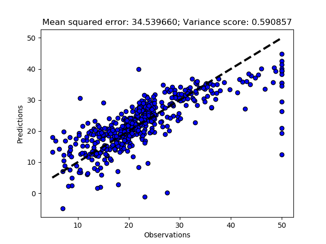
The complete function for implementing an iterative cross validation using folds, including writing out the regression coefficient and plotting.
    def MultiRegressionKfoldModel(self,folds=10, plot=True):
        regr = LinearRegression()
        #Set the kfold
        kfold = model_selection.KFold(n_splits=folds)
        #cross_val_predict returns an array of the same size as `y` where each entry
        #is a prediction obtained by cross validation:
        predict = model_selection.cross_val_predict(regr, self.X, self.y, cv=kfold)
        #To retrieve regressions scores, use cross_val_score
        scoring = 'r2'
        r2 = model_selection.cross_val_score(regr, self.X, self.y, cv=kfold, scoring=scoring)
        #The correlation coefficient
        print('Regression coefficients: \n', r2)
        #The mean squared error
        print("Mean squared error: %.2f" \
            % mean_squared_error(self.y, predict))
        #Explained variance score: 1 is perfect prediction
        print('Variance score: %.2f' \
            % r2_score(self.y, predict))
        if plot:
            title = ('Mean squared error: %(rmse)2f; Variance score: %(r2)2f' \
                      % {'rmse':mean_squared_error(self.y, predict),'r2': r2_score(self.y, predict)} )
            self.PlotRegr(self.y, predict, title, color='blue')
The complete code of the module that you created in this post is hidden under the button below, and available at GitHub.
Resources
SciKit learn Linear Regression Example
SciKit Plotting Cross-Validated Predictions
Your First Machine Learning Project in Python Step-By-Step by Jason Brownlee
Spot-Check Regression Machine Learning Algorithms in Python with scikit-learn by Jason Brownlee
Simple and Multiple Linear Regression in Python by Adi Bronshtein
Train/Test Split and Cross Validation in Python by Adi Bronshtein
Join And Merge Pandas Dataframe
Completed python module on GitHub.