Introduction
This post illustrates how to use Karttur’s GeoImagine Framework for plotting time series data. The commands and alternatives available for plotting the climate indexes time series data are the same also for plotting other time series data.
Prerequisites
You must have setup the Karttur’s GeoImagine Framework as described in earlier posts. You must also have added the climate indexes to the database.
The plotting functions of Karttur’s GeoImagine Framework make use of matplotlib, that can be called either as part of a Pandas DataFrame, or used directly. Plotting using Pandas DataFrame does not require any special parameters (the Framework relies completely on the default).
Framework process
The process for plotting climate indexes (and other database recorded) time series in Karttur’s GeoImagine Framework is plotdbtsancillary.
Process commands
All time series plotting can be done by using the Pandas package built in plot command. You simply do that by setting the parameter pdplot to True.
<?xml version='1.0' encoding='utf-8'?>
<plotdbtsclimate>
	<userproj userid = 'karttur' projectid = 'karttur' tractid= 'karttur-trmm' siteid = '*' plotid = '*' system = 'ancillary'></userproj>
	<period startyear = "1998" startmonth='01' endyear = "2017" endmonth='12' timestep='M'></period>
	<process processid = 'plotdbtsclimate' version = '1.3'>
		<parameters pdplot='True'></parameters>
		<index id ='soi'></index>
		<index id ='pdo'></index>
	</process>
</plotdbtsclimate>
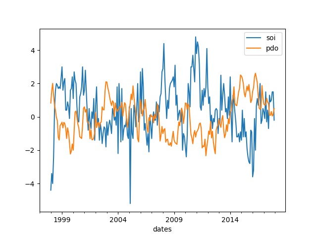
The xml commands above generate a plot with the two climate indexes, as shown below (soi = Southern Oscillation Index, pdo = Pacific Decadal Oscillation).
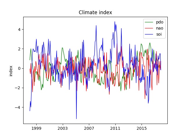
If you instead set pdplot to False, you can add title and axis, and decide the colors and styles of the included time series. Additionally you can also decide the size and resolution of the plot (see the reference page for plotdbtsclimate).
<?xml version='1.0' encoding='utf-8'?>
<plotdbtsclimate>
	<userproj userid = 'karttur' projectid = 'karttur' tractid= 'karttur-trmm' siteid = '*' plotid = '*' system = 'ancillary'></userproj>
	<period startyear = "1998" startmonth='01' endyear = "2017" endmonth='12' timestep='M'></period>
	<process processid = 'plotdbtsclimate' version = '1.3'>
		<parameters pdplot='True' title='Climate index'></parameters>
    <parameters pdplot='False' title='Climate index' legend='0' obslinestyle='solid' ylabel='index'></parameters>
		<index id ='pdo' obsformat = 'g-' ></index>
		<index id ='nao' obsformat = 'r-' ></index>
		<index id ='soi' obsformat = 'b-' ></index>
	</process>
</plotdbtsclimate>
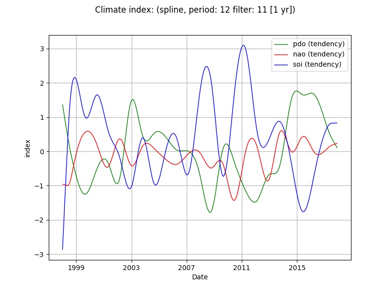
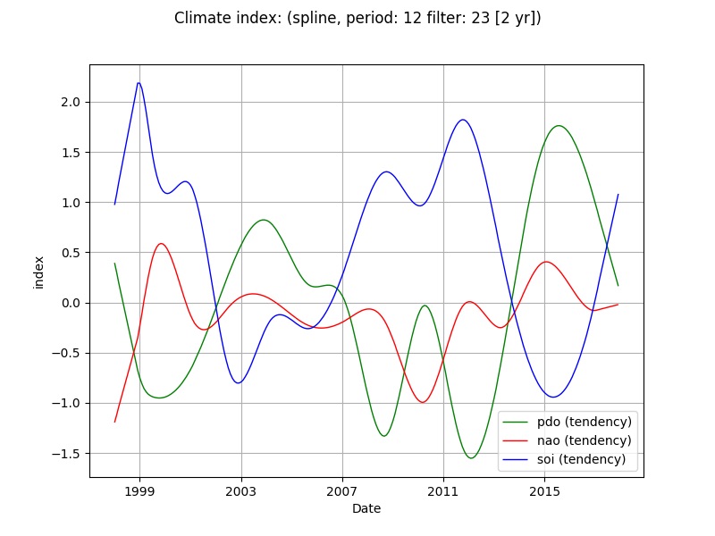
You can also do a time series decomposition on the fly, and display the smoothed time series (tendency) of several indexes in a single plot.
<?xml version='1.0' encoding='utf-8'?>
<plotdbtsclimate>
	<userproj userid = 'karttur' projectid = 'karttur' tractid= 'karttur-trmm' siteid = '*' plotid = '*' system = 'ancillary'></userproj>
	<period startyear = "1998" startmonth='01' endyear = "2017" endmonth='12' timestep='M'></period>
	<process processid = 'plotdbtsclimate' version = '1.3'>
  <parameters
  ylabel='index'
  title='Climate index'
  decompose='True'
  legend='0'
  grid='True'
  ></parameters>
  <index id ='pdo' obsformat = 'g-' tendencyformat = 'g-' trendformat = 'k-'></index>
  <index id ='nao' obsformat = 'r-' tendencyformat = 'r-' trendformat = 'k-'></index>
  <index id ='soi' obsformat = 'b-' tendencyformat = 'b-' trendformat = 'k-'></index>
	</process>
</plotdbtsclimate>
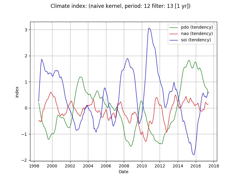
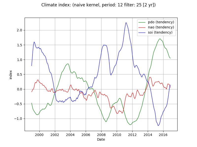
By default time series decomposition uses a spline functions for smoothing and removing the seasonal signal, as described in another post. The default size of the smoothing filter (kernel) equals the number of annual observations (i.e. 12 for monthly data), but can be set to any multiple of that number (with the parameter yearfac). Alternatively the smoothing can be done with a filter kernel (by setting the boolean parameter naive to True), commonly referred to as naive decomposition.
The figure below shows 4 single plots, all showing the smoothed time series (tendency). The top row shows the spline smoothed tendencies and the bottom row the naive tendencies. The left plots have been smoothed with a kernel representing a single (1) annual cycle, whereas the right plots have been smoothed using a kernel spanning 2 years. Note that the y-axis range differs between the plots.
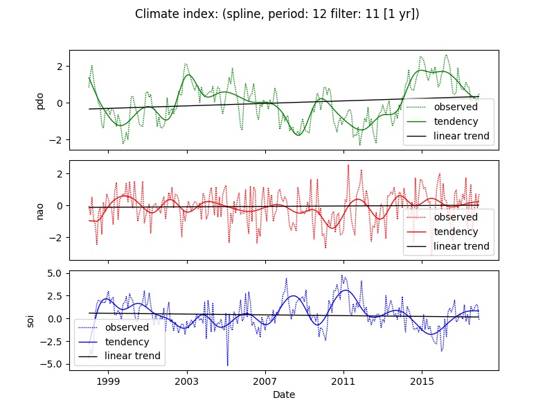
The last example shows how to plot multiple indexes as subplots in the same plot window.
<?xml version='1.0' encoding='utf-8'?>
<plotdbtsclimate>
	<userproj userid = 'karttur' projectid = 'karttur' tractid= 'karttur-trmm' siteid = '*' plotid = '*' system = 'ancillary'></userproj>
	<period startyear = "1998" startmonth='01' endyear = "2017" endmonth='12' timestep='M'></period>
	<process processid = 'plotdbtsclimate' version = '1.3'>
  <parameters
  title='Climate index'
  decompose='True'
  plotoriginal='True'
  plottrend='True'
  legend='0'
  separate='True'
  ></parameters>
  <index id ='pdo' obsformat = 'g-' tendencyformat = 'g-' trendformat = 'k-'></index>
  <index id ='nao' obsformat = 'r-' tendencyformat = 'r-' trendformat = 'k-'></index>
  <index id ='soi' obsformat = 'b-' tendencyformat = 'b-' trendformat = 'k-'></index>
	</process>
</plotdbtsclimate>
Project file
The project file is the same as used for importing climate indexes, but with one (1) additional link to the xml file defining the plots shown above (projFN = ‘/doc/ClimateIndexes/xml/climateIndexes-0800_plot.xml’):
from geoimagine.kartturmain.readXMLprocesses import ReadXMLProcesses, RunProcesses

if __name__ == "__main__":

    verbose = True

    #projFN = '/doc/ClimateIndexes/xml/climateIndex-0100_import-NOAA.xml'
    #projFN = '/doc/ClimateIndexes/xml/climateIndex-0100_import-co2records.xml'
    projFN = '/doc/ClimateIndexes/xml/climateIndexes-0800_plot.xml'

    procLL = ReadXMLProcesses(projFN,verbose)

    RunProcesses(procLL,verbose)
The linked xml contains the plot processes shown above, plus some more alternatives.
Resources
Linestyles (the linestyles implemented in the Framework)