Introduction
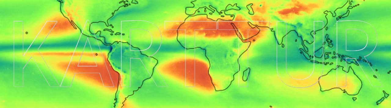
This post illustrates how to use Karttur’s GeoImagine Framework for calculating the Transformed Wetness Index (TWI) from Moderate Resolution Imaging Spectroradiometer (MODIS) spectral images.
Prerequisites
To follow this tutorial the previous post on accessing, downloading and organizing MODIS data must be completed.
Transformed Wetness Index (TWI)
The Transformed Wetness Index (TWI) is a non-linear normalized difference index that uses biophysical vectors representing the soil line and water derived from an orthogonal linear transformation of multi-spectral reflection data. I have used TWI for mapping global tropical wetlands and also for wetland change detection.
Project module
The project module file (projMODIS.py) is available in the Project package projects.
MODIS TWI calculations
Calculating TWI soil moisture (vol/vol) from MODIS reflectance bands requires three processes:
- Orthogonal transformation of the bands
- Scale preserved rotation and transformation
- Convert TWI to percent soil moisture
Orthogonal transformation
The MODIS image reflectance data (see previous post) can be used for classical statistical image classifications, or e.g. machine learning classification. But Karttur’s GeoImagine Framework also contains a module for deterministic, rather than statistical, modeling. The deterministic modeling package define linear transformations of the reflectance data to a biophysical feature space. In the remote sensing jargon, this is sometimes referred to as Tasseled Cap Transformation (TCT). Usually a TCT is based on fixed transformations coefficients, but in Karttur’s GeoImagine Framework you can also create your own, customized and calibrated, thematic transformation for classification of specific features.
Here I will only illustrate how to implement a pre-defined linear transformation. The processes for transforming MODIS reflectance data to a biophysical feature space are LinearTransformMODISRegion and LinearTransformMODISSingleTile.
The number of biophysical features can not exceed the number of bands. In the example below, two biophysical features are produced, tc-soil and tc-wet. Note that these two features are defined for optimizing the separation of wet and dry areas and are not defined as the original TCT features Brightness and Wetness.
Scale preserved rotation and transformation
Many of the classical indexes used in satellite image processing are derived from a normalized rationing:
index = (bandA - bandB) / (bandA + bandB)
including the Normalized Difference Vegetation Index (NDVI), the ND Snow Index (NDSI) and the several version of the ND Water Index (NDWI). Especially NDVI has been extensively applied for vegetation mapping and monitoring. More elaborate VI’s also use information from other bands, or adjustment factors, for reducing biases caused by e.g. atmospheric disturbances or soil backgrounds. A variety of different VI’s are implement in Karttur’s GeoImagine Framework. But the Framework also contains a more generic indexing tool, developed from Jack Paris Grand Unified Vegetation Index (GRUVI). The tool, however, can be used for indexing any surficial biophysical feature, not only vegetation.
In this post, you will implement the Transformed Wetness Index, which uses the tc-soil and tc-wet features as input. For a full reference to the method, see Gumbricht (2018).
Convert TWI to percent soil moisture
In my article on TWI I use an empirical algorithm for translating TWI from reflectance factor units to percent soil moisture. The formula is a scalar transformaion, and is implemented in the Framework as twipercentmodisRegion and twipercentmodisSingleTile.
The process setting up the conversion to percent above scales the output between 0 and 200, and thus has a scalefac = 2.
Seasonal signal extraction
The time series of the Transformed Wetness Index (TWI), created in the previous section, is plagued with gaps, in particular over regions with heavy cloud cover during the wet season(s). For reconstructing an unbiased annual signal you need to fill the gaps prior to any temporal resampling. To fill the gaps, you first need to extract the multiyear seasonal signal.
The processes extractseasonmodisRegion and extractseasonmodisSingleTile extracts the seasonal multiyear signal. You can only give the source composition (<srccomp>) in this process.
The extractseasonModis processes do not accept any destination composition (<dstcomp>). The naming and composition of the destination tine series is defaulted, and can not be manually set. The format of the seasonal layers will be exactly the same as the original time series. The seasonal layers will be stored under a thematic folder with the same name as the original time series, but with the suffix “-sesn”. The file naming will also be identical, except for the date part, that will be changed to the format:
“startyear”-“endyear”@”seasonalperiod”
The seasonal files resulting from the xml file above will thus have the date parts like: 2001-2017@D009, 2001-2017@D026 … etc.
Filling missing data
As noted in the previous section, the MODIS data have large gaps, and I choose to fill these gaps prior to analyzing trends and changes (and prior to creating animations). The processes for filling MODIS data gaps are seasonfilltsModisRegion and seasonfilltsModisSingleTile.
The process xml command only requires the composition for the original time series. But the process expects that the corresponding seasonal signals (for the given period and timestep) already exist. Remember that the naming of the seasonal layers is defaulted, and can not be set. The seasonfilltsModis processes fill in all missing records in the original time series using a combination of interpolation and the average seasonal signal for the same period that filled.
The previous date, whether observed or interpolated itself, is always given a weight of 0.5. The remaining weight fraction (0.5) is divided between the next observation and the average seasonal signal. The closer in time the next observation, the higher the weight. By default, the weight for the next observation value is determined by the formula:
weight = 1.4/(distance)**2+3.0)
resulting in the following default weights:
| Distance to next | Weight previous | Weight next | Weight seasonal |
|---|---|---|---|
| 0 | 0.5 | 0.47 | 0.03 |
| 1 | 0.5 | 0.35 | 0.15 |
| 2 | 0.5 | 0.2 | 0.3 |
| 3 | 0.5 | 0.12 | 0.38 |
| 4 | 0.5 | 0.07 | 0.43 |
| 5 | 0.5 | 0.05 | 0.45 |
Note that the previous period can itself be a result of an interpolation, in which case the seasonal signal and the next period have already influenced the previous period value.
Time series export and animation
After running the process seasonfilltsModis and the conversion to percent soil moisture, you should have a complete time series of 16D interval MODIS estimated percent soil moisture (TWI) layers. In my example here, I have included all years from 2001 to 2017, or 17 years. To create the animation I need to define a clock/timeline layout, the movie frame size, and if and how to emboss the finished movie. The post on SMAP processing contains a more detailed step-by-step tutorial on how to create layouts for spatial data and the movieclock.
Add movieclock
I will illustrate using two example (further down). The first is the MODIS tile h20v10, covering the wetlands of central southern Africa. To avoid covering the Okavango Inland Delta in Northern Botswana, I have to put the clock in the lower right corner. To do that I define a movieclock using all the default settings, but with the clock position set to the lower right (lr) corner:
<?xml version='1.0' encoding='utf-8'?>
<palette>
	<userproj userid = 'karttur' projectid = 'karttur' tractid= 'karttur' siteid = '*' plotid = '*' system = 'system'></userproj>
	<!-- addmovieclock -->
	<process processid = 'addmovieclock'>
		<overwrite>Y</overwrite>
		<delete>N</delete>
		<parameters name = 'twilr'
		position = 'lr'
		>
		</parameters>
	</process>
</palette>
TWI palette and scaling
I also need a palette for the TWI (soil moisture) data. The palette is set reflecting the range of the TWI percent (from 0 to 200) data.
<?xml version='1.0' encoding='utf-8'?>
<palette>
	<userproj userid = 'karttur' projectid = 'karttur' tractid= 'karttur' siteid = '*' plotid = '*' system = 'system'></userproj>
	<!-- addrasterpalette twi-->
	<process processid = 'addrasterpalette'>
		<parameters palette = 'twi' compid='test'>
			<setcolor id = '0' red = '255' green ='132' blue='94' alpha ='0' label='0' hint='0' ></setcolor>
			<setcolor id = '25' red = '240' green ='224' blue='148' alpha ='0' label='10' hint='NA' ></setcolor>
			<setcolor id = '50' red = '162' green ='162' blue='122' alpha ='0' label='50' hint='no correlation' ></setcolor>
			<setcolor id = '100' red = '70' green ='89' blue='112' alpha ='0' label='100' hint='positive correclation' ></setcolor>
			<setcolor id = '150' red = '20' green ='60' blue='210' alpha ='0' label='150' hint='positive correclation' ></setcolor>
			<setcolor id = '200' red = '2' green ='1' blue='190' alpha ='0' label='200' hint='strong positive correlation' ></setcolor>
			<setcolor id = '250' red = '2' green ='1' blue='190' alpha ='0' label='250' hint='strong positive correlation' ></setcolor>
			<setcolor id = '253' red = '245' green ='237' blue='182' alpha ='0' label='dry (0)' hint='completely dry' ></setcolor>
			<setcolor id = '254' red = '32' green ='32' blue='32' alpha ='255' label='frame' hint='frame' ></setcolor>
			<setcolor id = '255' red = '250' green ='250' blue='250' alpha ='255' label='255' hint='no data' ></setcolor>
		</parameters>
	</process>
</palette>
Also a scaling is needed, even if the scaling in this case is a direct 1:1 relation.
<?xml version='1.0' encoding='utf-8'?>
<scaling>
	<userproj userid = 'karttur' projectid = 'karttur' tractid= 'karttur' siteid = '*' plotid = '*' system = 'system'></userproj>
	<!-- Create scaling -->
	<process processid = 'createscaling' version = '1.3'>
		<parameters scalefac='1' mirror0='False'></parameters>
		<comp id = '1' source = "MCD43A4v006" product = "MCD43A4" folder = "twi-fill-percent" band = "twipercent" prefix = "twipercent" suffix = "v006-tg01">	</comp>
    	<comp id = '2' source = "MCD43A4v006" product = "MCD43A4" folder = "twi-percent" band = "twipercent" prefix = "twipercent" suffix = "v006-tg01">	</comp>
	</process>
</scaling>
Export
Once you have creates the palette and scaling for the MODIS TWI percent composition, you can export the data as color images (maps). The scaling can not be set in the exporttobytesmap process. It must be given in the database and related to the data to be exported using the theme (folder) and name (band) of the layer. The palette to use must be set as a parameter.
<?xml version='1.0' encoding='utf-8'?>
<export>
	<userproj userid = 'karttur' projectid = 'karttur' tractid= 'karttur' siteid = '*' plotid = '*' system = 'modis'></userproj>
	<period startyear = '2001' endyear = '2017' timestep='16D'></period>
	<process processid ='exporttobyteModisSingleTile' dsversion = '1.3'>
		<overwrite>True</overwrite>
		<parameters palette='twi' htile='20' vtile='10'></parameters>
		<srcpath volume = "Karttur3tb"></srcpath>
		<dstpath volume = "Karttur3tb"></dstpath>
		<srccomp>
			<TWIpercent id='TWI' source = "MCD43A4v006" product = "MCD43A4" folder = "TWI-fill-percent" band = "TWIpercent" prefix = "TWIpercent" suffix = "v006-tg01">
			</TWIpercent>
		</srccomp>
	</process>
</export>
The export processes always exports the data using the same projection and the spatial resolution as the source data. When exporting the data for layout and mapping, the cell format is changed to Byte (0-255).
MODIS TWI animation
To create animations based on the the MODIS sinusoidal tiles, you need to run the two processes movieframeModisSingleTile and movieclockModisSingleTile. The post on SMAP processing contains a more detailed step-by-step tutorial on how to create animations from time series images.
The first process, movieframeModisSingleTile, creates the movie frames. By default it creates a shell script file, reported when process finished, that that you must run. For the MODIS tiles herein, I set the frame dimensions to 800800 (rather than the original 24002400). The movies are thus smaller compared to the original data.
<?xml version='1.0' encoding='utf-8'?>
<runprocess>
	<userproj userid = 'karttur' projectid = 'karttur' tractid= 'karttur' siteid = '*' plotid = '*' system = 'modis'></userproj>
	<period startyear = "2001" endyear = "2017"  timestep='16D'></period>

	<process processid = 'movieframeModisSingleTile' version = '1.3'>
		<parameters framewidth = '800' framecrop='800,800,0,0' emboss='KARTTUR' embossdims='720,150' embossptsize='100' htile='20' vtile='10'></parameters>
		<srcpath volume = "karttur3tb" hdrfiletype = 'tif' datfiletype = 'tif'></srcpath>
		<dstpath volume = "/Volumes/karttur3tb/movieclock" hdrfiletype = 'png' datfiletype = 'png'></dstpath>
		<srccomp>
			<TWIpercent id='TWI' source = "MCD43A4v006" product = "MCD43A4" folder = "TWI-fill-percent" band = "TWIpercent" prefix = "TWIpercent" suffix = "v006-tg01">
			</TWIpercent>
		</srccomp>
	</process>
</runprocess>
The second process, movieclockModisSingleTile, creates one clock image per movie frame. It then also creates two shell script files, one for overlaying the clock frames over the movie frames, and one for generating the movies. You have to run both manually as explained in the post on SMAP processing
<?xml version='1.0' encoding='utf-8'?>
<runprocess>
	<userproj userid = 'karttur' projectid = 'karttur' tractid= 'karttur' siteid = '*' plotid = '*' system = 'modis'></userproj>
	<period startyear = "2001" endyear = "2017"  timestep='16D'></period>

	<process processid = 'movieclockModisSingleTile' version = '1.3'>
		<overwrite>True</overwrite>
		<parameters clocklayout = 'twilr' moviewidth = '800' htile='20' vtile='10'></parameters>
		<dstpath volume = "/Volumes/karttur3tb/movieclock" hdrfiletype = 'png' datfiletype = 'png'></dstpath>
		<dstcomp>
			<TWIpercent id='TWI' source = "MCD43A4v006" product = "MCD43A4" folder = "TWI-fill-percent" band = "TWIpercent" prefix = "TWIpercent" suffix = "v006-tg01">
			</TWIpercent>
		</dstcomp>
	</process>
</runprocess>