Machine learning 5 - Dimension reduction

Contents - introduction - Prerequistits - Skeleton - Methods for dimension reduction - Agglomeration - Model hyper-parameterization - Principal Component Analysis (PCA) - Resources

introduction

In earlier posts in this series on machine learning, you have applied both linear and non-linear regressors for predictive modelling. In the post on feature selection different methods for discriminating among the independent features aiming at retaining only the most adequate is applied. In this post you will instead rearrange the independent variables and create a novel set of independent variables reducing the dimensionality (number of columns) while retaining more of the variation. The methods presented in this post are considered more powerful than simply discriminating among the independent variables.

You can copy and paste the code in the post, but you might have to edit some parts: indentations does not always line up, quotations marks can be of different kinds and are not always correct when published/printed as html text, and the same also happens with underscores and slashes.

The complete code is also available here.

Prerequistits

The prerequisites are the same as in the previous posts in this series: a Python environment with numpy, pandas, sklearn (Scikit learn) and matplotlib installed.

Module Skeleton

The module skeleton code is under the button.


  
import numpy as np
import pandas as pd
from sklearn import model_selection
from sklearn import linear_model
from sklearn.neighbors import KNeighborsRegressor
from sklearn.tree import DecisionTreeRegressor
from sklearn.ensemble import RandomForestRegressor
from sklearn.svm import SVR
from sklearn.metrics import mean_squared_error, r2_score

import matplotlib
matplotlib.use(‘TkAgg’)
from matplotlib import pyplot

class RegressionModels:
    ‘'’Machinelearning using regression models
    ‘’’
    def __init__(self, columns,target):
        ‘'’creates an instance of RegressionModels
        ‘’’
        self.columns = columns
        self.target = target
        #create an empty dictionary for features to be discarded by each model
        self.modelDiscardD = {}

def ImportUrlDataset(self,url):    
    self.dataframe = pd.read_csv(url, delim_whitespace=True, names=self.columns)

def ExtractDf(self,omitL):
    #extract the target column as y
    self.y = self.dataframe[target]
    #appeld the target to the list of features to be omitted
    omitL.append(self.target)
    #define the list of data to use
    self.columnsX = [item for item in self.dataframe.columns if item not in omitL]
    #extract the data columns as X
    self.X = self.dataframe[self.columnsX]

def PlotRegr(self, obs, pred, title, color='black'):
    pyplot.xticks(())
    pyplot.yticks(())
    fig, ax = pyplot.subplots()
    ax.scatter(obs, pred, edgecolors=(0, 0, 0),  color=color)
    ax.plot([obs.min(), obs.max()], [obs.min(), obs.max()], 'k--', lw=3)
    ax.set_xlabel('Observations')
    ax.set_ylabel('Predictions')
    pyplot.title(title)
    pyplot.show()

def ModelSelectSet(self,modD):
    self.models = []
    if 'OLS' in modD:
        self.models.append(('OLS', linear_model.LinearRegression(\*\*modD['OLS'])))
        self.modelDiscardD['OLS'] = []
    if 'TheilSen' in modD:
        self.models.append(('TheilSen', linear_model.TheilSenRegressor(\*\*modD['TheilSen'])))
        self.modelDiscardD['TheilSen'] = []
    if 'Huber' in modD:
        self.models.append(('Huber', linear_model.HuberRegressor(\*\*modD['Huber'])))
        self.modelDiscardD['Huber'] = []
    if 'KnnRegr' in modD:
        self.models.append(('KnnRegr', KNeighborsRegressor( \*\*modD['KnnRegr'])))
        self.modelDiscardD['KnnRegr'] = []
    if 'DecTreeRegr' in modD:
        self.models.append(('DecTreeRegr', DecisionTreeRegressor(\*\*modD['DecTreeRegr'])))
        self.modelDiscardD['DecTreeRegr'] = []
    if 'SVR' in modD:
        self.models.append(('SVR', SVR(\*\*modD['SVR'])))
        self.modelDiscardD['SVR'] = []
    if 'RandForRegr' in modD:
        self.models.append(('RandForRegr', RandomForestRegressor( \*\*modD['RandForRegr'])))
        self.modelDiscardD['RandForRegr'] = []

def RegrModTrainTest(self, testsize=0.3, plot=True):
    #Split the data into training and test substes
    X_train, X_test, y_train, y_test = model_selection.train_test_split(self.X, self.y, test_size=testsize)
    #Loop over the defined models
    for m in self.models:
        #Retrieve the model name and the model itself
        name,mod = m
        #Remove the features listed in the modelDiscarD
        self.ExtractDf(self.modelDiscardD[name])
        #Fit the model
        mod.fit(X_train, y_train)
        #Predict the independent variable in the test subset
        predict = mod.predict(X_test)
        #Print out the model name
        print 'Model: %s' %(name)
        #Print out RMSE
        print("    Mean squared error: %.2f" \
            % mean_squared_error(y_test, predict))
        #Print explained variance score: 1 is perfect prediction
        print('    Variance score: %.2f' \
            % r2_score(y_test, predict))
        if plot:
            title = ('Model: %(mod)s; RMSE: %(rmse)2f; r2: %(r2)2f' \
                      % {'mod':name,'rmse':mean_squared_error(y_test, predict),'r2': r2_score(y_test, predict)} )
            self.PlotRegr(y_test, predict, title, color='green')

def RegrModKFold(self,folds=10, plot=True):
    #set the kfold
    kfold = model_selection.KFold(n_splits=folds)
    for m in self.models:
        #Retrieve the model name and the model itself
        name,mod = m
        #Remove the features listed in the modelDiscarD
        self.ExtractDf(self.modelDiscardD[name])
        #cross_val_predict returns an array of the same size as `y` where each entry
        #is a prediction obtained by cross validation:
        predict = model_selection.cross_val_predict(mod, self.X, self.y, cv=kfold)
        #to retriece regressions scores, use cross_val_score
        scoring = 'r2'
        r2 = model_selection.cross_val_score(mod, self.X, self.y, cv=kfold, scoring=scoring)
        #The correlation coefficient
        #Print out the model name
        print 'Model: %s' %(name)
        #Print out correlation coefficients
        print('    Regression coefficients: \n', r2)    
        #Print out RMSE
        print("Mean squared error: %.2f" \
              % mean_squared_error(self.y, predict))
        #Explained variance score: 1 is perfect prediction
        print('Variance score: %.2f' \
            % r2_score(self.y, predict))
        if plot:
            title = ('Model: %(mod)s; RMSE: %(rmse)2f; r2: %(r2)2f' \
                      % {'mod':name,'rmse':mean_squared_error(self.y, predict),'r2': r2_score(self.y, predict)} )
            self.PlotRegr(self.y, predict, title, color='blue')

def RandomTuningParams(self,nFeatures):
    self.paramDist = {}
    # specify parameters and distributions to sample from
    for m in self.models:
        name,mod = m
        print ('name'), (name), (mod.get_params())
        if name == 'KnnRegr':
            self.paramDist[name] = {"n_neighbors": sp_randint(4, 12),
                          'leaf_size': sp_randint(10, 50),
                          'weights': ('uniform','distance'),
                          'p': (1,2),
                          'algorithm': ('auto','ball_tree', 'kd_tree', 'brute')}
        elif name =='DecTreeRegr':
            self.paramDist[name] = {"max_depth": [3, None],
                          "min_samples_split": sp_randint(2, 6),
                          "min_samples_leaf": sp_randint(1, 4)}
        elif name =='SVR':
            self.paramDist[name] = {"kernel": ['linear', 'rbf'],
                          "epsilon": (0.05, 0.1, 0.2),
                          "C": (1, 2, 5, 10)}
        elif name =='RandForRegr':
            self.paramDist[name] = {"max_depth": [3, None],
                          "n_estimators": sp_randint(10, 50),
                          "max_features": sp_randint(1, nFeatures),
                          "min_samples_split": sp_randint(2, 6),
                          "min_samples_leaf": sp_randint(1, 5),
                          "bootstrap": [True,False]}

def RandomTuning(self, fraction=0.5, nIterSearch=6, n_top=3):
    #Randomized search
    for m in self.models:
        #Retrieve the model name and the model itself
        name,mod = m
        print name, self.paramDist[name]
        search = RandomizedSearchCV(mod, param_distributions=self.paramDist[name],
                                           n_iter=nIterSearch)
        X_train, X_test, y_train, y_test = model_selection.train_test_split(self.X, self.y, test_size=(1-fraction))
        search.fit(X_train, y_train)
        self.ReportSearch(search.cv_results_,n_top)
        #Retrieve the top ranked tuning
        best = np.flatnonzero(search.cv_results_['rank_test_score'] == 1)
        tunedModD=search.cv_results_['params'][best[0]]
        #Append any initial modD hyper-parameter definition
        for key in self.modD[name]:
            tunedModD[key] = self.modD[name][key]
        regmods.modD[name] = tunedModD

def ReportModParams(self):
    print 'Model hyper-parameters:'
    for m in self.models:
        #Retrieve the model name and the model itself
        name,mod = m
        print ('    name'), (name), (mod.get_params())


if __name__ == (‘__main__’):
    columns = [‘CRIM’, ‘ZN’, ‘INDUS’, ‘CHAS’, ‘NOX’, ‘RM’, ‘AGE’, ‘DIS’, ‘RAD’, ‘TAX’, ‘PTRATIO’, ‘B’, ‘LSTAT’, ‘MEDV’]
    target = ‘MEDV’
    regmods = RegressionModels(columns, target)
    regmods.ImportUrlDataset(‘https://archive.ics.uci.edu/ml/machine-learning-databases/housing/housing.data’)
```

Methods for dimension reduction

This post covers two different methods for reducing the dimensions in the independent variables:

Feature agglomeration
Principle Component Analysis (PCA)

Import the required packages from Scikit learn.

from sklearn.cluster import FeatureAgglomeration
from sklearn.decomposition import PCA

For the feature agglomeration you are going to use a pipeline approach for setting up a selection model, and then sending the model to the grid search module GridSearchCV that you used in the previous post. For that you also need to import the Scikit learn modules for BayesianRidge (the model to use for agglomeration), Pipeline and Memory. And then you also need to import GridSearchCV and RandomizedSearchCV.

from sklearn.linear_model import BayesianRidge
from sklearn.pipeline import Pipeline
from sklearn.externals.joblib import Memory
from sklearn.model_selection import GridSearchCV
from sklearn.model_selection import RandomizedSearchCV

Agglomeration

Agglomeration aims at reducing the dimensionality (number of columns) of the independent (X) data by merging features that show similar variation patterns. The clustering function in Scikit learn FeatureAgglomeration uses the Ward hierarchical cluster analysis, and clusters the original X dimension to n_clusters. Add the function WardClustering to the RegressionsModels class.

    def WardClustering(self, nClusters):
        ward = FeatureAgglomeration(n_clusters=nClusters)
        #fit the clusters
        ward.fit(self.X, self.y)
        #print out the clustering
        print 'labels_', ward.labels_
        #Reset self.X
        self.X = ward.transform(self.X)
        #print the shape of reduced X data
        print 'Agglomerated X data shape:',self.X.shape

The function resets the class X (self.X) variable, and all subsequent processing (regression modelling) will use the clustered data instead of the original data. Your models will then have fewer independent features to sieve through. The modelling will thus be faster, but with only a small loss in predictive power, and without redundancy among the independent features.

When calling the WardClustering function you have to give the number of clusters you want to merge the original dataset into. To use the function, call it from the __main__ section.

    nClusters = 5
    regmods.WardClustering(nClusters)
    #Processes called after the clustering will use the clustered X dataset for modelling
    #Setup regressors to test
    regmods.modD['KnnRegr'] = {}
    regmods.modD['DecTreeRegr'] = {}
    regmods.modD['SVR'] = {}
    regmods.modD['RandForRegr'] = {}

    #Invoke the models
    regmods.ModelSelectSet()

    #set the random tuning parameters
    regmods.RandomTuningParams()
    #Run the tuning
    regmods.RandomTuning()
    #Reset the models with the tuned hyper-parameters
    regmods.ModelSelectSet()
    #Run the models
    regmods.RegrModTrainTest()
    regmods.RegrModKFold()   

With the __main__ section set as above the module:

agglomerates the X data to 5 clusters,
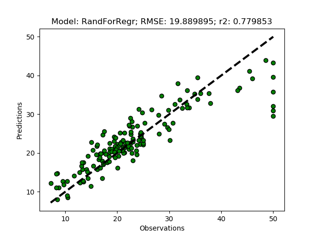
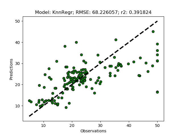
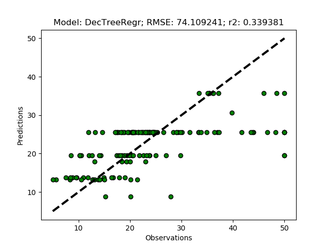
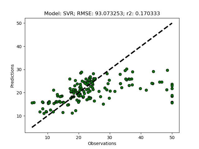
sets up 4 regressors (‘KnnRegr, ‘DecTreeRegr’, ‘SVR’ and ‘RandForRegr’),
uses a randomized tuning for setting the model hyper-paramters for each regressor, and
test the predictive powers of each regressor using both train+test and cross validation.

It will take a while.

Tuning the number of clusters

In the section above we set an arbitrary number (5) defining the number of clusters that we wanted our dataset to be merged into. To tune an optimal number of clusters we could (manually) change the parameter nClusters and check the result for each trial. But it would be much better to set up a process using a grid search evaluating different alternative agglomerations. In the previous post you used GridSearchCV for finding the best hyper-parameters. GridSearchCV can also be used for identifying the optimal number of clusters. But you must set it up so that GridSearchCV has some criterion on which to base the search for the optimal nClusters.

What is needed for tuning the optimal number of clusters is an estimator (regressor) that evaluates the effects of different nClusters. You thus need a process that:

iteratively changes nClusters,
agglomerates X into nClusters using WardClustering,
sends the clustered X dataset to an estimator, and
evaluates the results from the estimator.

In Scikit learn this can be setup using a pipeline (Pipeline) and GridSearchCV. Pipeline defines the functions to link, and GridSearchCV defines the cluster sizes to test and iterates the process. The example below uses the Bayesian linear regressor as the estimator, and is taken from a Scikit learn page on Feature agglomeration.

    def TuneWardClustering(self, nClustersL, kfolds=2):
        print 'Cluster agglomereations to test',nClustersL
        cv = KFold(kfolds)  # cross-validation generator for model selection
        ridge = BayesianRidge()
        cachedir = tempfile.mkdtemp()
        mem = Memory(cachedir=cachedir)
        ward = FeatureAgglomeration(n_clusters=6, memory=mem)
        clf = Pipeline([('ward', ward), ('ridge', ridge)])
        # Select the optimal number of parcels with grid search
        clf = GridSearchCV(clf, {'ward__n_clusters': nClustersL}, n_jobs=1, cv=cv)
        clf.fit(self.X, self.y)  # set the best parameters
        print 'initial Clusters',iniClusters
        #report the top three results
        self.ReportSearch(clf.cv_results_,3)
        #rerun with the best cluster agglomeration result
        return (clf.best_params_['ward__n_clusters'])

The function TuneWardClustering requires a list (nClustersL) containing the sizes of the clusters you want to test (for example, to test clustering the X data to between 4 and 10 cluster, the list would be [4,5,6,7,8,9,10]). You can also set the number of folds (kfolds) to use in the cross validation. The function returns a single number, the number of clusters that resulted in the highest score.

You then also need to add the reporting function for the results of the pipeline clustering.

    def ReportSearch(self, results, n_top=3):
        for i in range(1, n_top + 1):
            candidates = np.flatnonzero(results['rank_test_score'] == i)
            for candidate in candidates:
                print("Model with rank: {0}".format(i))
                print("Mean validation score: {0:.3f} (std: {1:.3f})".format(
                      results['mean_test_score'][candidate],
                      results['std_test_score'][candidate]))
                print("Parameters: {0}".format(results['params'][candidate]))
                print("")

When running the module you can choose to explore the results, or you can just send the best clustering results (the returned parameter from TuneWardClustering) to the function WardClustering.

To test the agglomeration function for exploring the results of the feature agglomeration, update the __main__ section.

    #nClusters = 5
    #Agglomerate the X data
    nClustersL = [4,5,6,7,8,9,10,11]
    nClusters = regmods.TuneWardClustering(nClustersL)
    regmods.WardClustering(nClusters)
    '''
    #Processes called after the clustering will use the clustered X dataset for modelling
    #Setup regressors to test
    regmods.modD['KnnRegr'] = {}
    regmods.modD['DecTreeRegr'] = {}
    regmods.modD['SVR'] = {}
    regmods.modD['RandForRegr'] = {}

    #Invoke the models
    regmods.ModelSelectSet()

    #set the random tuning parameters
    regmods.RandomTuningParams()
    #Run the tuning
    regmods.RandomTuning()
    #Reset the models with the tuned hyper-parameters
    regmods.ModelSelectSet()
    #Run the models
    regmods.RegrModTrainTest()
    regmods.RegrModKFold()
    '''

If you kept the suggested parameters, the results should be that the best option is to use 6 clusters.

Model with rank: 1
Mean validation score: 0.441 (std: 0.100)
Parameters: {'ward__n_clusters': 6}

Model with rank: 2
Mean validation score: 0.435 (std: 0.029)
Parameters: {'ward__n_clusters': 9}

Model with rank: 3
Mean validation score: 0.415 (std: 0.075)
Parameters: {'ward__n_clusters': 7}

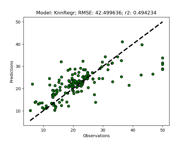
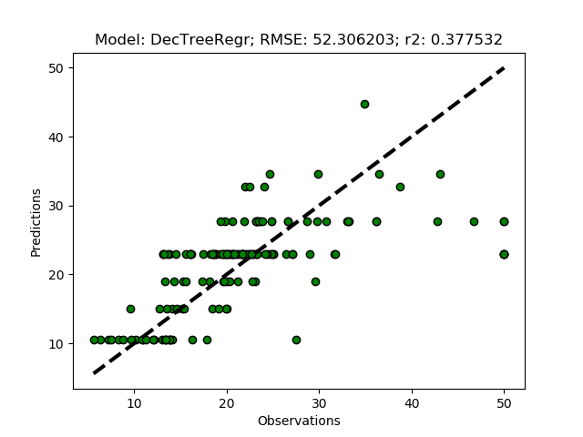
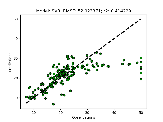
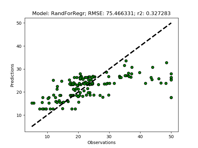
To run the models with the suggested number of clusters, just remove the commented section invoking the models (the triple quotations '''). The module then runs both the training+test model predictions RegrModTrainTest) and the folded cross validation predictions RegrModKFold). All models are tuned before actually running the predictions, hence it will take a while for the model formulations to finish and the first plot to appear.

Comparison of predictions from various regressors after feature agglomeration (to 6 clusters) and randomized hyper-parameter tuning.

Principal Component Analysis (PCA)

PCA is a linear transformation that places a set of n-vectors (called eigen-vectors) sequentially oriented orthogonally with regard to previously defined vectors, while seeking an orientation that maximizes the explanation of the remaining variation. The maximum number of vectors that can be constructed equals the number of input features, whereafter all the variation in the original data is explained by the vectors. The information content decreases with each vector, and usually the 3 to 4 first components carry almost all information from the original dataset.

You already imported the PCA function from Scikit learn above, to implement the PCA dimension reduction add the function PCAdecompose to the RegressionModels class.

    def PCAdecompose(self, minExplainRatio=0, nComps=3 ):
        if minExplainRatio > 0:
            pca = PCA()
            pca.fit(self.X)
            print 'PCA explained ratios', pca.explained_variance_ratio_
            nComps = len([item for item in pca.explained_variance_ratio_ if item >= minExplainRatio])
            print 'accepted components: %(n)d' %{'n':nComps}
        pca = PCA(n_components=nComps)
        pca.fit(self.X)
        self.X = pca.transform(self.X)
        print 'PCA explained ratios', pca.explained_variance_ratio_
        print 'PCA X data shape:',self.X.shape

By default PCAdecompose reduces the input array to three principal components. Alternatively you can either set a threshold for the ratio of the total variation that a component must explain to be accepted (minExplainRatio), or set the number of components to be constructed (nComps). For the latter to be used, you must set the former to zero (0). To run your regressors using eigen-vectors from PCA as the independent variables, just replace the agglomeration with PCA in the __main__ section.

    '''
    #Agglomerate the X data
    nClustersL = [4,5,6,7,8,9,10,11]
    nFeatures = regmods.TuneWardClustering(nClustersL)
    regmods.WardClustering(nClusters)
    '''
    #Dimension reduction using PCA
    nFeatures = regmods.PCAdecompose() #default: produces 3 eigen-vectors
    #nFeatures = regmods.PCAdecompose(0.1) #produces all eigen-vectors that explain at least 10% of the total variation
    #nFeatures = regmods.PCAdecompose(0, 4) #produces 4 eigen-vectors

    #Setup regressors to test
    regmods.modD['KnnRegr'] = {}
    regmods.modD['DecTreeRegr'] = {}
    regmods.modD['SVR'] = {}
    regmods.modD['RandForRegr'] = {}

    #Invoke the models
    regmods.ModelSelectSet()

    #set the random tuning parameters
    regmods.RandomTuningParams(nFeatures)
    #Run the tuning
    regmods.RandomTuning()
    #Reset the models with the tuned hyper-parameters
    regmods.ModelSelectSet()
    #report model settings
    regmods.ReportModParams()
    #Run the models
    regmods.RegrModTrainTest()
    regmods.RegrModKFold()