This post presents the graphical results of the analysis of the correlations between water input (rainfall or Vertical Water Balance [VWB]) and water storage (equivalent water pillar depth) for Sub-Saharan Africa. The processing for deriving the images and movies are presented in the previous post.
Master vs slave movies
The movies below have the master (rainfall or VWB) as a smaller inset overlaying the slave (Earth’s equivalent water pillar). All three movies clearly illustrate how the Intertropical Convergence Zone (ITCZ) governs the rainfall pattern, with the equivalent water pillar seemingly lagging behind. This is perhaps most clearly seen in the movie with the total VWB as master (the second movie).
Rainfall as master
Total VWB as master
Surplus VWB as master
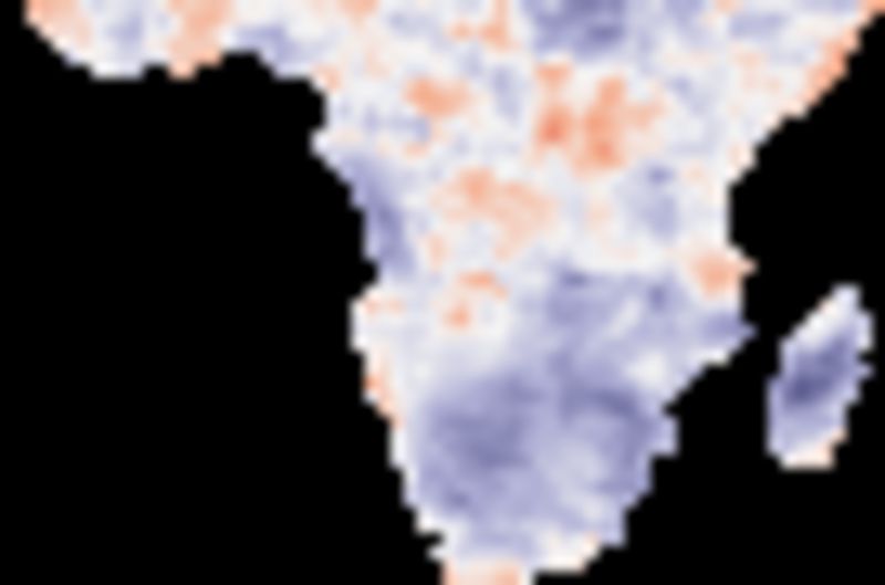
Trend comparisons
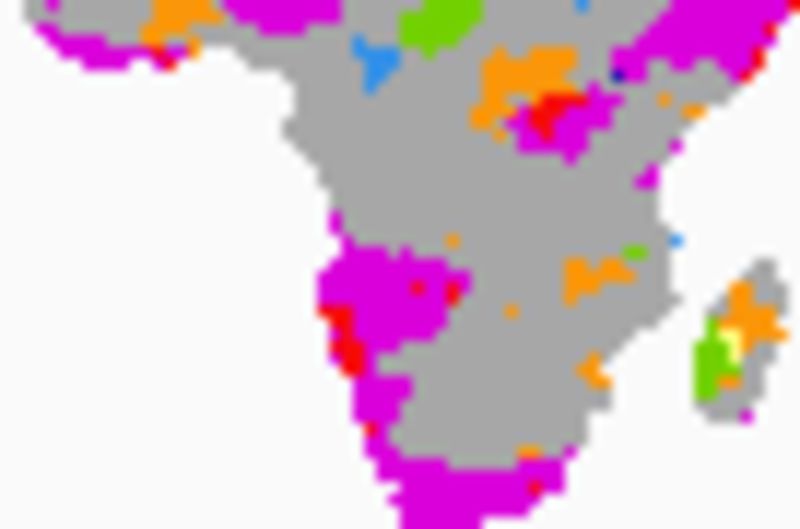
The comparison of trends in the figure below shows the congruence of the directions of significant (p<0.05) changes. The maps use the 9 classes defined in the method post. The left panel shows the congruence between significant changes in rainfall and equivalent water pillar depth; the right panel the changes in surplus VWB and equivalent water pillar depth. The total VWB result is identical to the result for rainfall.

Cross correlation water input vs water storage
The cross correlations capture the statistical relations of the movies above.
Observed cross correlations
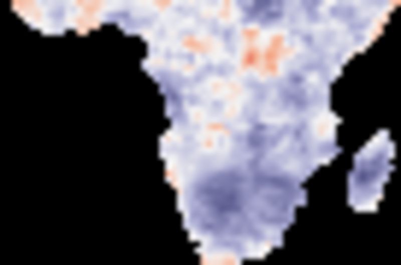
The figure below shows the best lag and the corresponding Pearson number for observed (not decomposed) datasets. The slave (dependent) is the same in all panels: the equivalent water pillar depth depth estimates. From top to bottom the masters (drivers) are: rainfall, total VWB and surplus VWB.


The cross correlation results are almost identical when comparing rainfall and total VWB as the master or driver. The cross correlations then adopting surplus VWB as the driver are either equal to, or worse, compared to using total VWB (or rainfall).
Decomposed cross correlations of rainfall
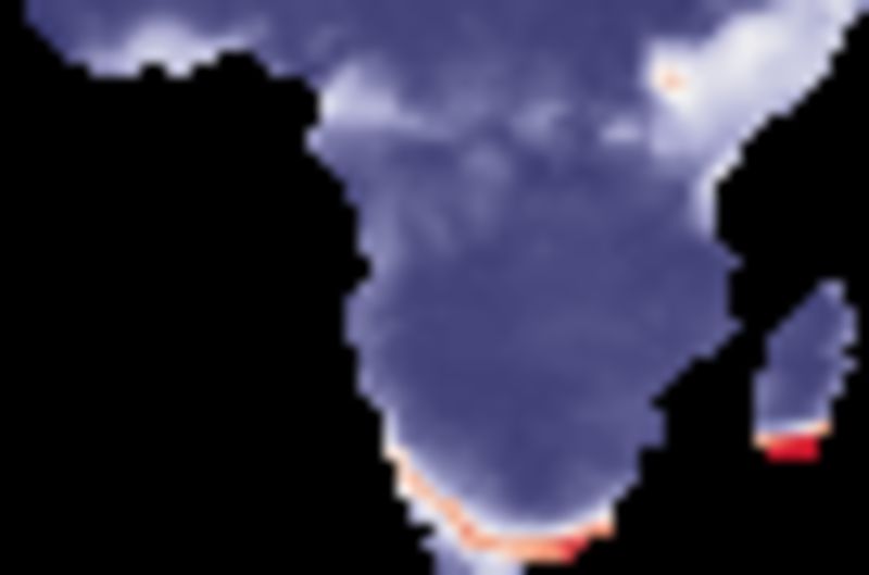
The figure shows the best lag and the corresponding Pearson number for rainfall as master and equivalent water pillar depth as slave for three different time series components: top) season, center) trend (or tendency) and, bottom) residual.


The cross correlations for the decomposed data show highly varying results for the different components. The seasonal signals of rainfall and equivalent water pillar depth are highly correlated except along the equator and at some coastal regions. The lag between the rainfall and water pillar is between 1 and 2 months (see figure below). The correlation between the trends (tendencies) are strongly varying, including regions with negative correlations and with dominating longer lag times (see figure below). The correlations between the residuals are weak, but positive and with a lag of 1 month dominating most of southern Africa (see below).
Seasonal lag correlations
The figure shows the Pearson number (correlation) for decomposed seasonal signals with rainfall as master and equivalent water pillar depth as slave, starting with no (0) lag and increasing with a lag of one month per map.


Trend lag correlations
The figure shows the Pearson number (correlation) for decomposed trends (tendencies) with rainfall as master and equivalent water pillar depth as slave, starting with no (0) lag and increasing with a lag of one month per map.


Residual lag correlations
The figure shows the Pearson number (correlation) for decomposed residual with rainfall as master and equivalent water pillar depth as slave, starting with no (0) lag and increasing with a lag of one month per map.