TRMM rainfall - results – Geo Imagine Developer

This post presents the graphical results of the analysis of Tropical Rainfall Measurement Mission (TRMM) rainfall for Sub-Saharan Africa. The processing for deriving the images and movies are presented in the previous post.

Monthly TRMM

The movie below is constructed from all the TRMM dates over Sub-Saharan Africa used in this project.

Monthly rainfall estimated from TRMM and other sources (TRMM product 3B43)

TRMM annual trends 1987-2017

The TRMM rainfall statistics and trends are calculated from annually aggregated data.

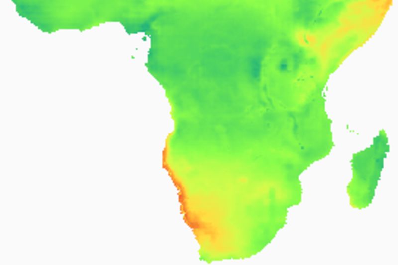
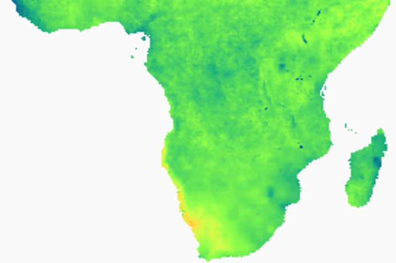
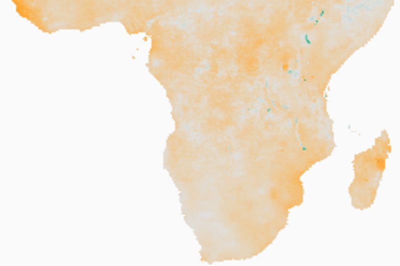
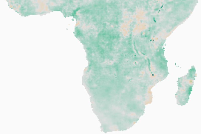
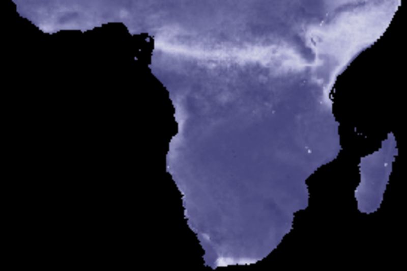
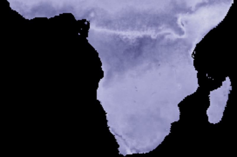
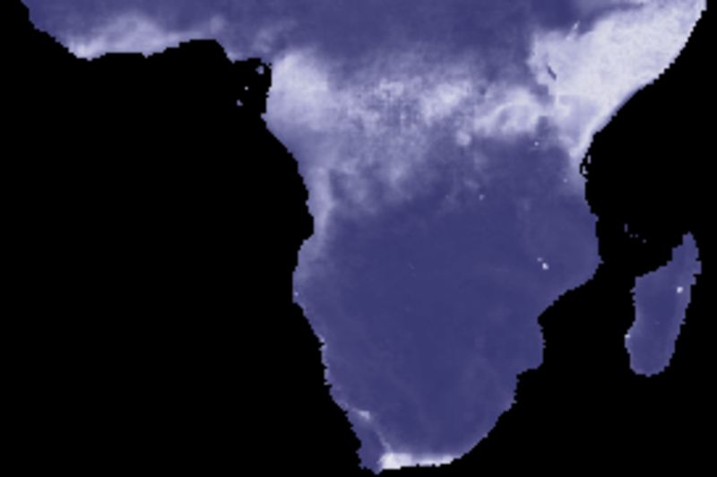
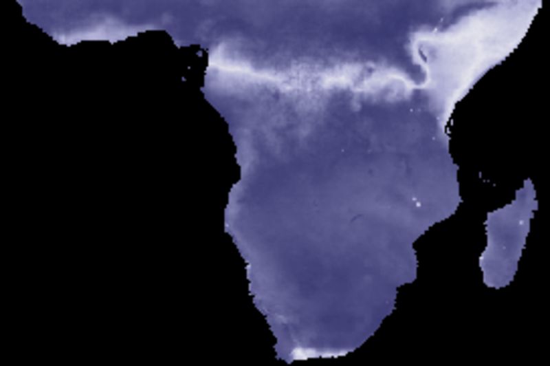
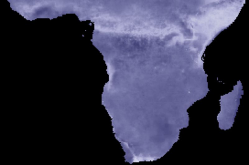
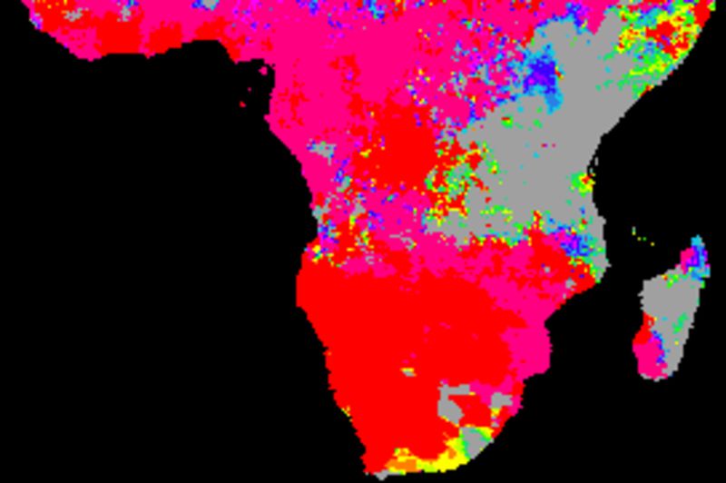
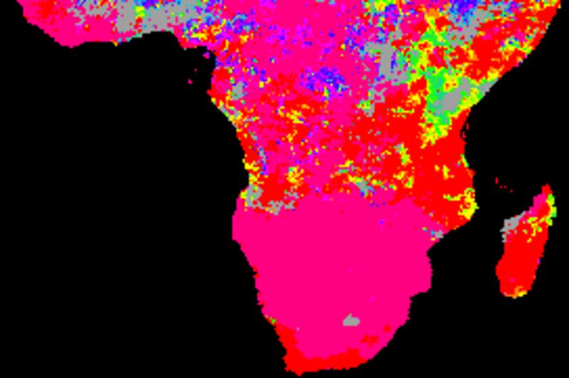
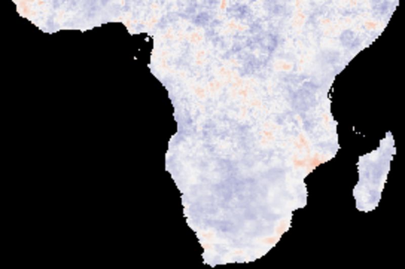
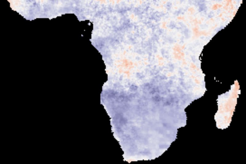
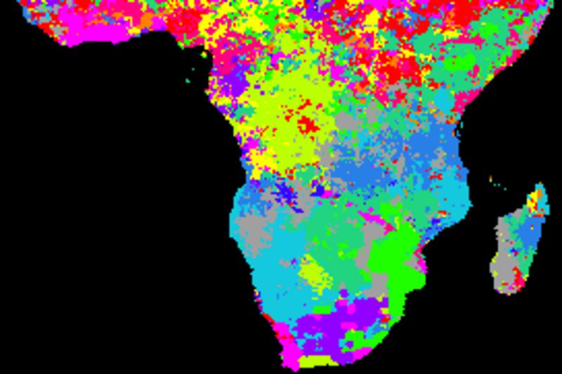
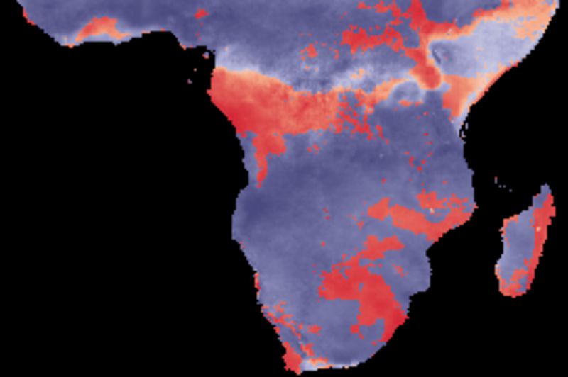
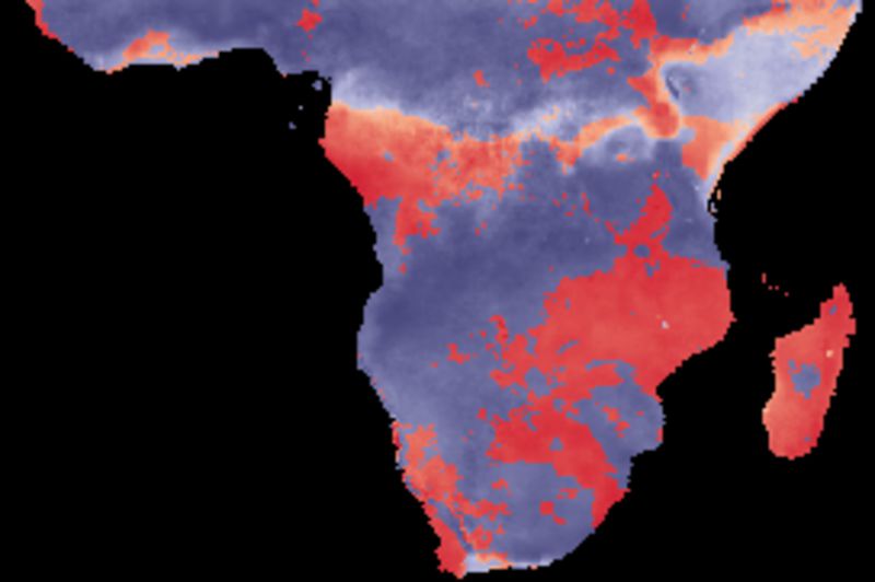
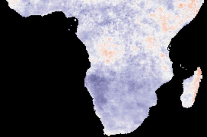
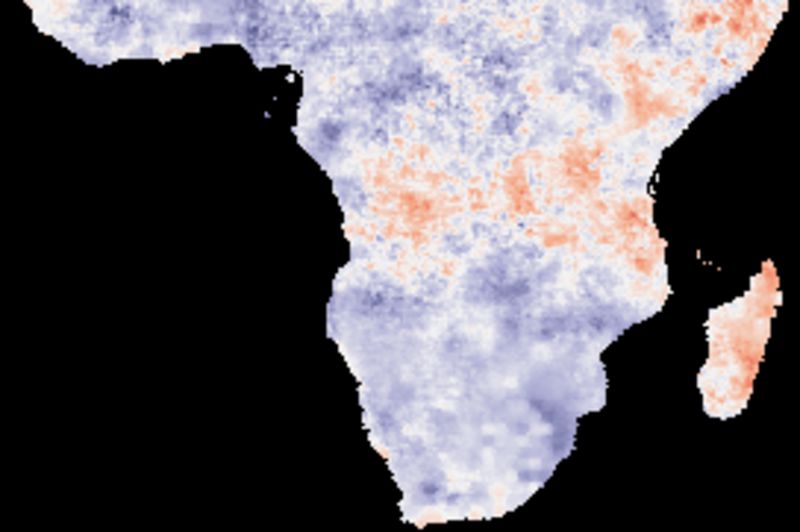
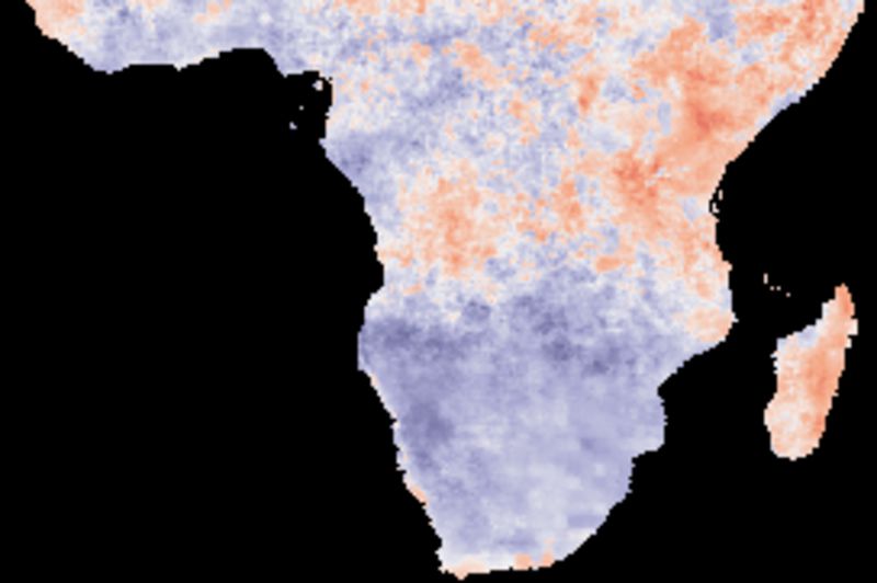
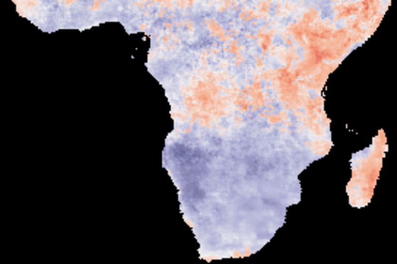
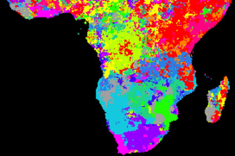
Rainfall mean and standard deviation

Rainfall over sub-saharan Africa estimated from TRMM for the period 1998 to 2017; the left panel shows average annual rainfall and the right standard deviation.

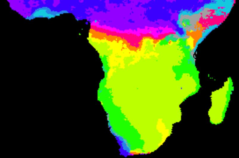
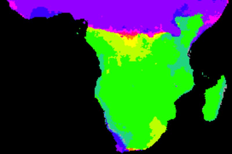
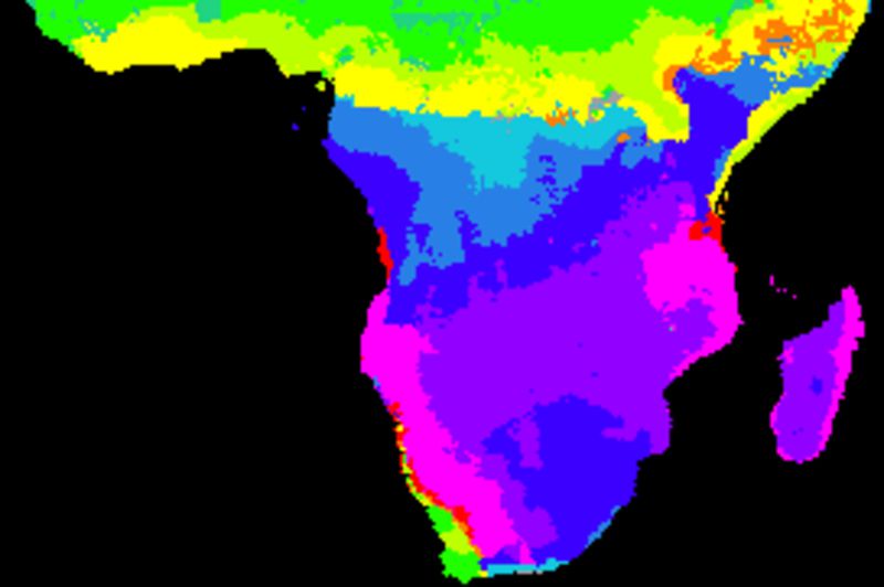
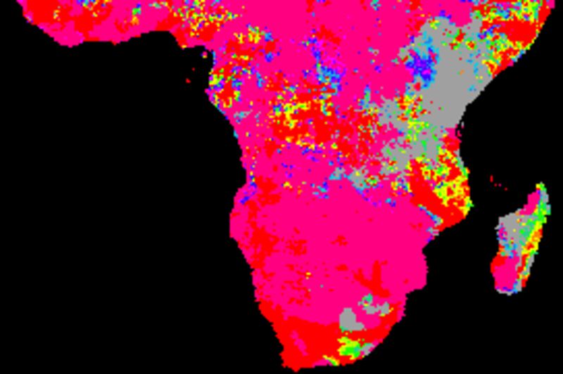
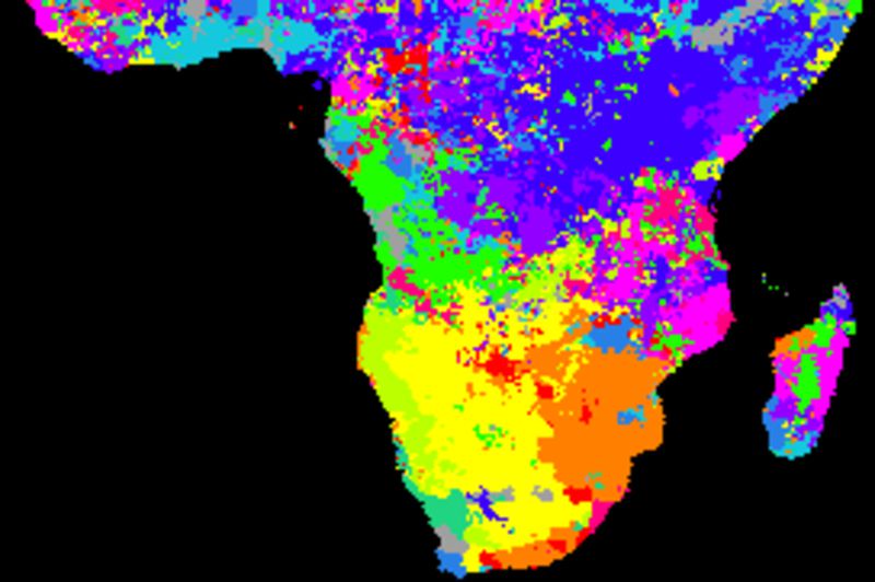
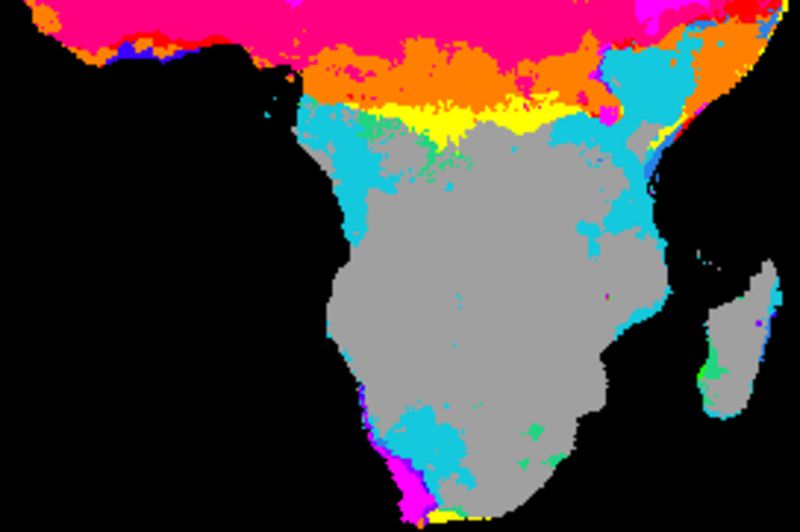
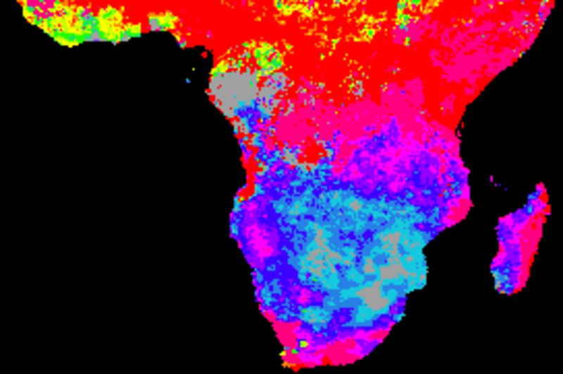
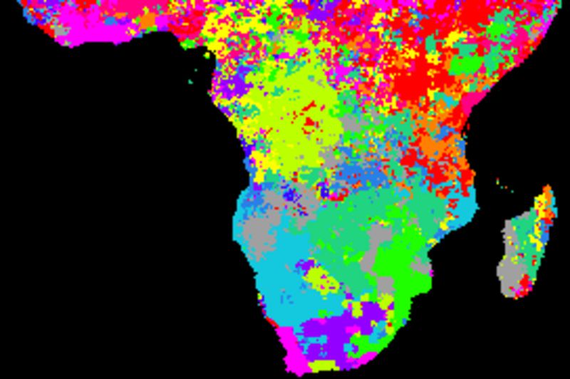
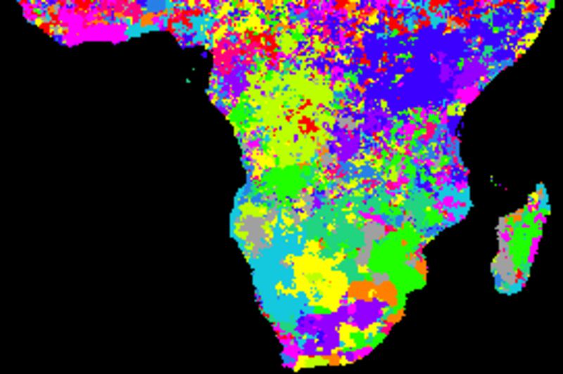
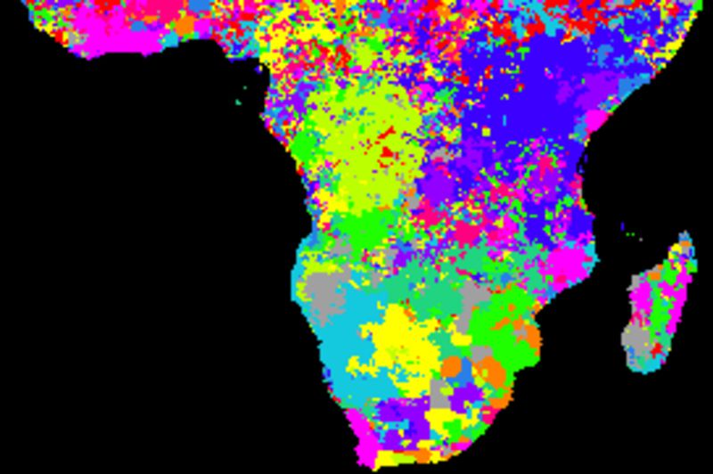
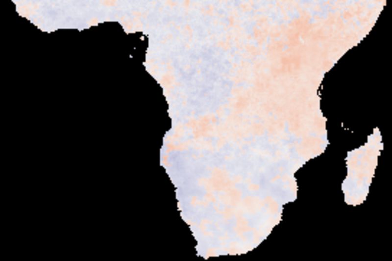
Rainfall trends

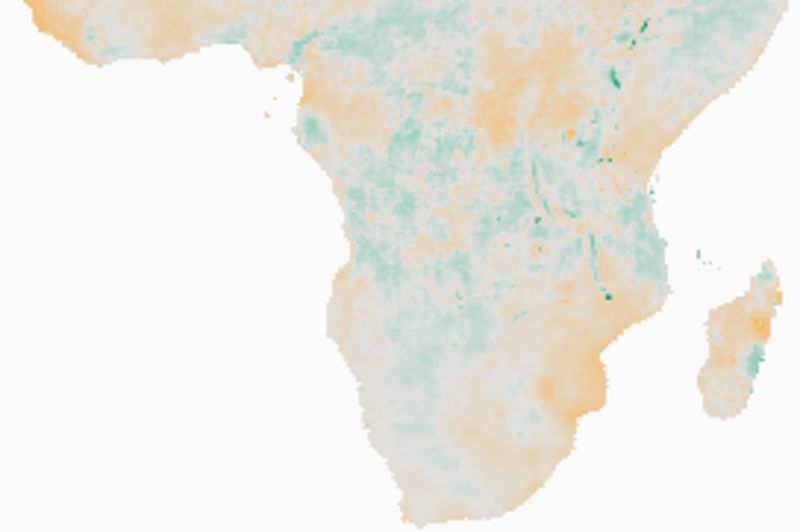
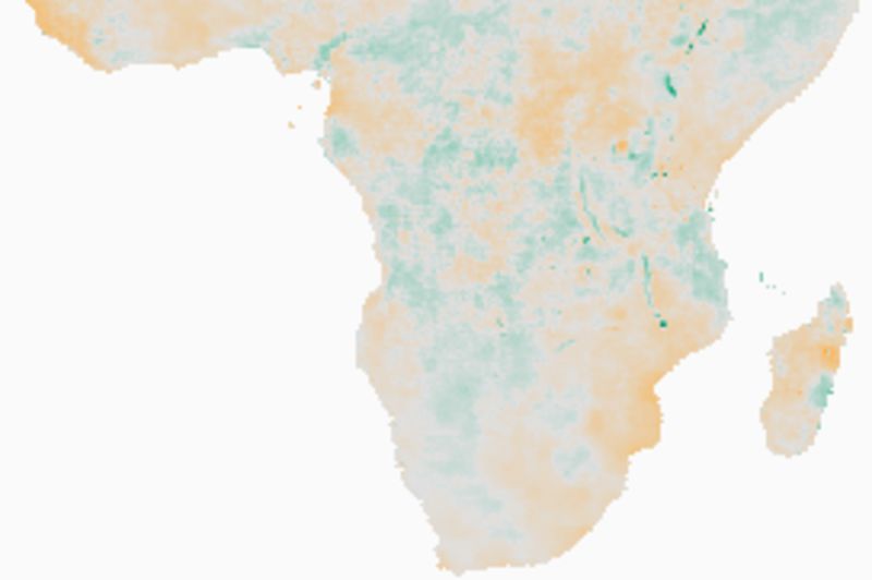
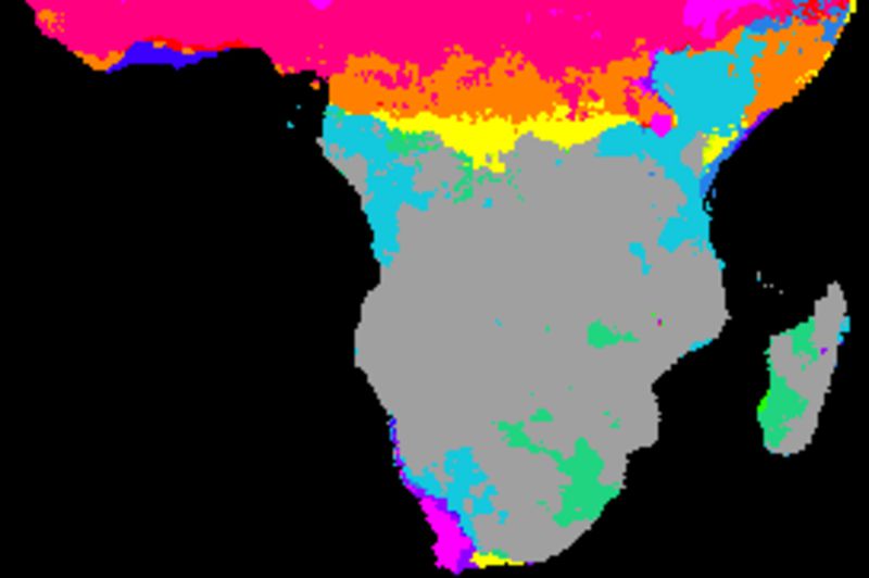
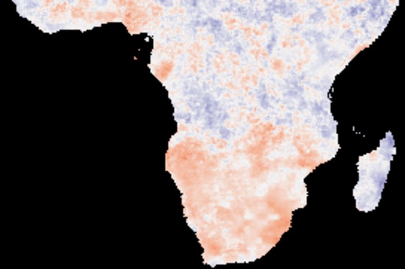
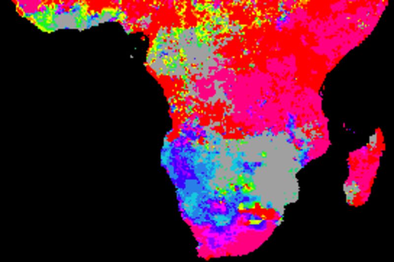
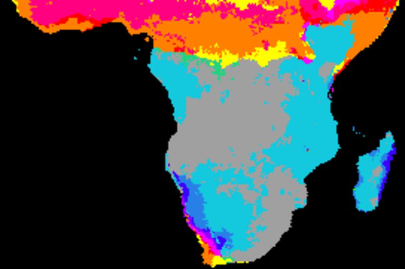
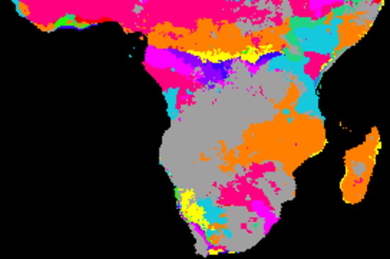
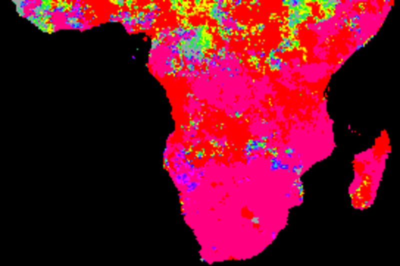
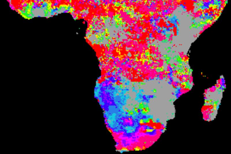
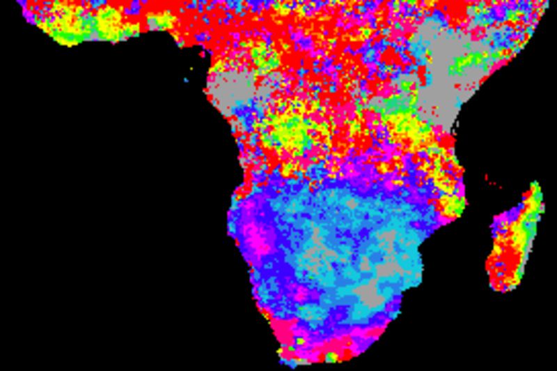
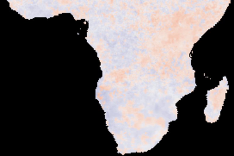
Comparison of rainfall regression model slopes as estimated from TRMM for the period 1998 to 2017; clockwise, starting with the upper left panel, the maps show ordinary least square (OLS), median Theil-Sen (TS), upper bound of the 95 % confidence interval of the median TS slope, and the lower left panel the lower bound of the 95 % confidence interval of the median TS slope.

Rainfall changes and significant trends

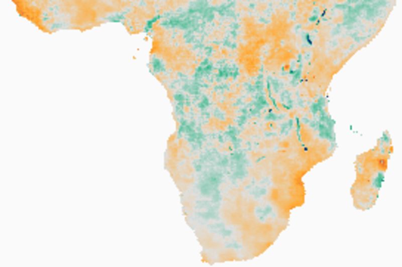
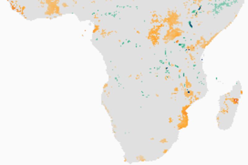
Estimated absolute changes in rainfall 1998 to 2017: the left panel shows the change for all regions, the right only changes where the Mann-Kendall test indicates significant changes (p<0.05).

Note how the estimates of the Theil-Sen 95 % confidence level fits well with the map of significant changes as estimated from the Mann-Kendall test. Regions that show a negative trend at the 95 % upper confidence interval of the TS are also indicated as areas with significant negative trend using the MK test.

Cross correlation climate indexes and TRMM

The cross correlations between global climate indexes and local rainfall can be done in many different ways. Perhaps the most important is to find the most relevant index for the study area. The first set of images below thus compare the cross correlations for the indexes used in this study:

BEST (Bivariate ENSO Timeseries ) (ENSO)
NAO (North Atlantic Oscillation) (Teleconnetions)
Nino3 (East Central Tropical Pacific SST) (ENSO, SST:Pacific)
PDO (Pacific Decadal Oscillation) (Teleconnetions)
PNA (Pacific North American Index) (Teleconnetions)
SOI (Southern Oscillation Index) (Atmosphere)

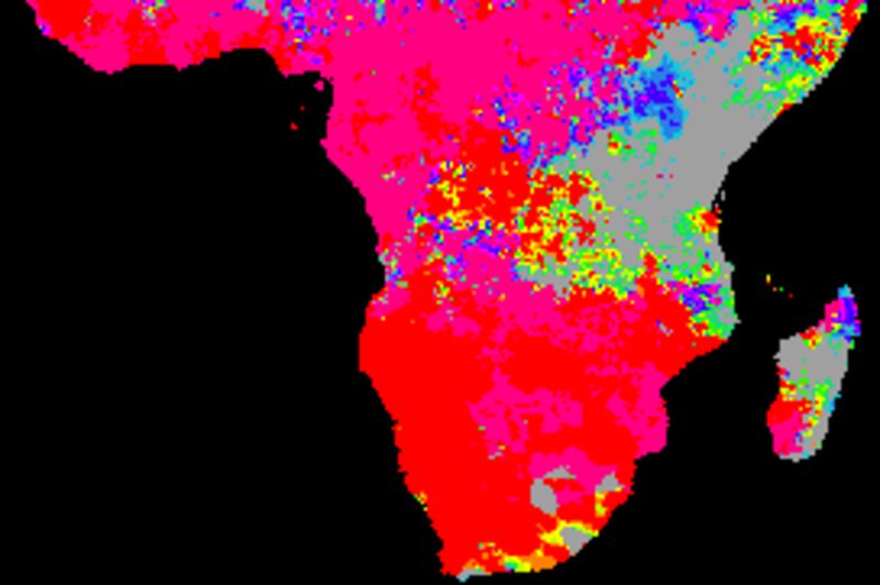
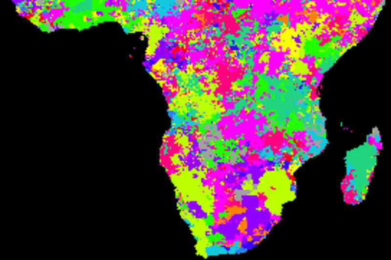
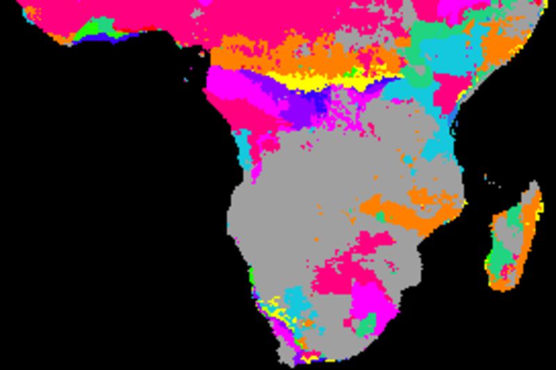
Index comparisons: season

The figure below shows cross correlations between the decomposed seasonal signal, derived from a naive (gliding mean) smoothing using an annual cycle (12 values). The climate indexes and each local pixel are smoothed and decomposed using the same method. The left panels show the lag with the highest correlation and the right panels the Pearson numbers of the best lag. From top to bottom the indexes are: BEST, NAO, Nino3, PDO, PNA and SOI.

Cross correlation of seasonal signals for six different climate indexes and local rainfall (TRMM). The left row shows the lag for the best correlation and right image the Pearson correlation for the best lag. From top to bottom the indexes are: BEST, NAO, Nino3, PDO, PNA and SOI.

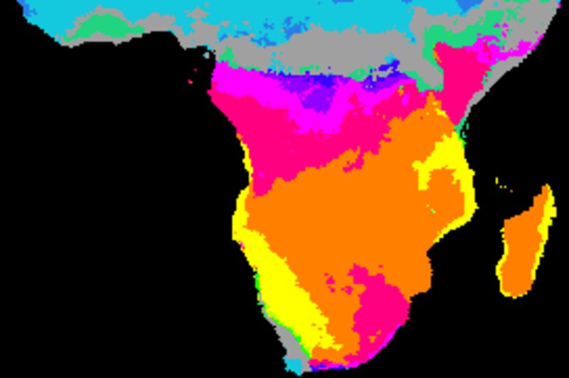
Except for NAO, the local seasonal rainfall is strongly related to global climate indexes for large parts of southern Africa. The correlations breaks down along the equator and at coastal regions, but are strong were the seasonal rainfall pattern is linked to the Intertropical Convergence Zone (ITCZ). The overall best local rainfall correlations are with two the El Nino Southern Oscillation (ENSO) indexes (BEST and Nina3), followed by the Pacific Decadal Oscillation (PDO).

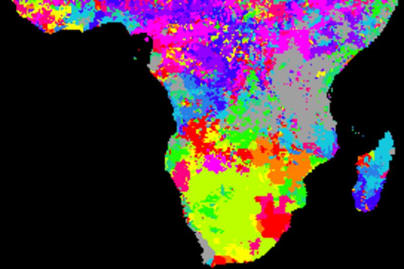
Index comparisons: tendency

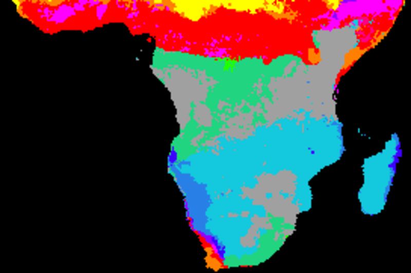
The figure below shows cross correlations between the decomposed trend (or tendency), derived from a naive (gliding mean) smoothing using an annual cycle (12 values). The climate indexes and each local pixel are smoothed and decomposed using the same method.

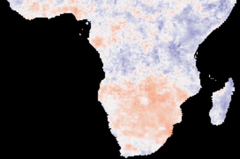
Cross correlation of smoothed tendency (trend) for six different climate indexes and local rainfall (TRMM). The left row shows the lag for the best correlation and right image the Pearson correlation for the best lag. From top to bottom the indexes are: BEST, NAO, Nino3, PDO, PNA and SOI.

Comparing the cross correlations between the long term (1998 to 2017) trends, the best performing indexes are PNA and SOI. The two ENSO indexes (BEST and Nina3) show dominantly negative correlations for large parts of southern Africa.

Index comparisons: residual

The figure below shows cross correlations between the decomposed residuals after removing the trends and seasonal signals derived from a naive (gliding mean) smoothing using an annual cycle (12 values). The climate indexes and each local pixel are smoothed and decomposed using the same method.

Cross correlation of decomposed residuals for six different climate indexes and local rainfall (TRMM). The left row shows the lag for the best correlation and right image the Pearson correlation for the best lag. From top to bottom the indexes are: BEST, NAO, Nino3, PDO, PNA and SOI.

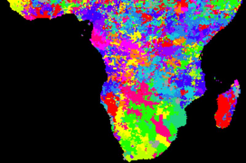
None of the indexes show consistent better or worse performance compared to the others. More elaborate studies, including applying different smoothing algorithms and kernel (filter) sizes and detailed analysis of the spatial distributions of the cross correlations are required.

Comparing smoothing algorithms

This section compares cross correlations applying different smoothing functions and kernel (filter) sizes. Based on the comparisons between the performance of the different climate indexes above, the SOI index is used for comparing smoothing algorithms. The following five different parameter settings are tested:

Naive kernel, 1 annual cycle (12 values)
Spline kernel, 1 annual cycle (12 values)
Spline kernel, 2 annual cycles (24 values)
Naive kernel, 1 annual cycle (12 values), absolute best correlation
Spline kernel, 1 annual cycle (12 values), absolute best correlation

The two last algorithms are identical to the first two, but accept the absolute best correlations between the climate index and the local rainfall. In effect this means that if the absolute negative correlation is higher than any positive correlations, that is accepted as the best performing. This reveals if the local rainfall is inversely related to the climate index.

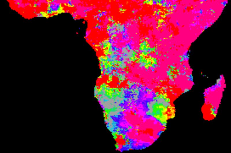
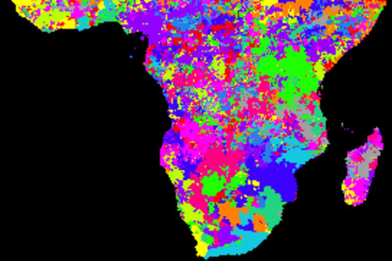
SOI seasonal correlations

The figure below shows cross correlations between decomposed seasonal signals and SOI using different smoothing algorithms. SOI and each local pixel are smoothed and decomposed using the same method in each comparison. The left panels show the lag with the highest correlation and the right panels the Pearson numbers of the best lag. Applied algorithms from top to bottom: naive kernel (1 yr), spline kernel (1 yr), spline kernel (2 yrs), absolute correlation naive kernel (1 yr), absolute correlation spline kernel (1 yr).

Cross correlation of seasonal trend for the Southern Oscillation Index (SOI) and local rainfall (TRMM). The left row shows the lag for the best correlation and right image the Pearson correlation for the best lag. The five rows show the results of using different smoothing functions for the time series decomposition, from top to bottom: naive kernel (1 yr), spline kernel (1 yr), spline kernel (2 yrs), absolute correlation naive kernel (1 yr), absolute correlation spline kernel (1 yr).

The correlation results with annual spanning naive kernel and spline are very similar (2 topmost panels). The larger filter size (2 years, mid panel) tends to give a lower correlation compared to using a filter size representing a single year. Some regions, especially at marginal positions and along the equator, show inverse correlations with SOI. The inverse correlations, however, are also associated with a large lag. This suggests that the seasonal rainfall is related to the integrated SOI signal representing a longer period.

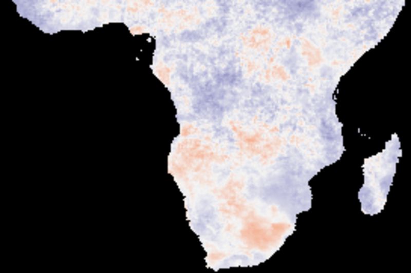
SOI tendency correlations

The figure below shows cross correlations between decomposed tendencies (trends) and SOI using different smoothing algorithms. SOI and each local pixel are smoothed and decomposed using the same method in each comparison. The left panels show the lag with the highest correlation and the right panels the Pearson numbers of the best lag. Applied algorithms from top to bottom: naive kernel (1 yr), spline kernel (1 yr), spline kernel (2 yrs), absolute correlation naive kernel (1 yr), absolute correlation spline kernel (1 yr).

The correlation results with annual spanning naive kernel and spline are very similar. The larger filter size (2 years, mid panels) tends to enhance (both negative and positive) correlations as compared to using a filter size representing a single year. Regions without any positive correlation (brown areas in the tree top panels) have stronger inverse correlations (two bottom panels).

SOI residual correlations

The figure below shows cross correlations between decomposed residuals after removing the trends and seasonal signals and SOI using different smoothing algorithms. SOI and each local pixel are smoothed and decomposed using the same method in each comparison. The left panels show the lag with the highest correlation and the right panels the Pearson numbers of the best lag. Applied algorithms from top to bottom: naive kernel (1 yr), spline kernel (1 yr), spline kernel (2 yrs), absolute correlation naive kernel (1 yr), absolute correlation spline kernel (1 yr).

The cross correlations between decomposed residual signals are weak and show no patterns when comparing the SOI index and local rainfall.