Machine learning 6 - Fit polynomials – Geo Imagine Developer

introduction

This post is an attempt to test Machine Learning for predicting soil properties from spectra data.

Prerequistits

The prerequisites are the same as in the previous posts in this series: a Python environment with numpy, pandas, sklearn (Scikit learn) and matplotlib installed.

Module Skeleton

The module skeleton code will be made avaialble.

The complete code of the module that you created in this post is available at GitHub.

Material and methods

The data used is from OSSL covering south central Sweden.

Results

NIR broadband models

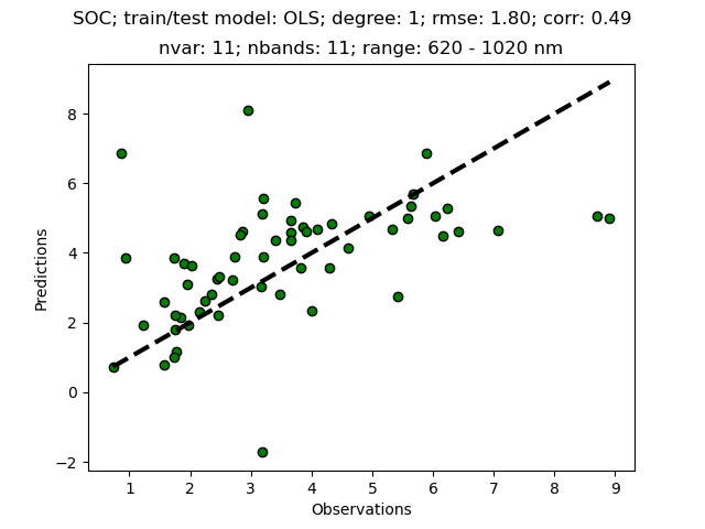
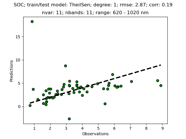
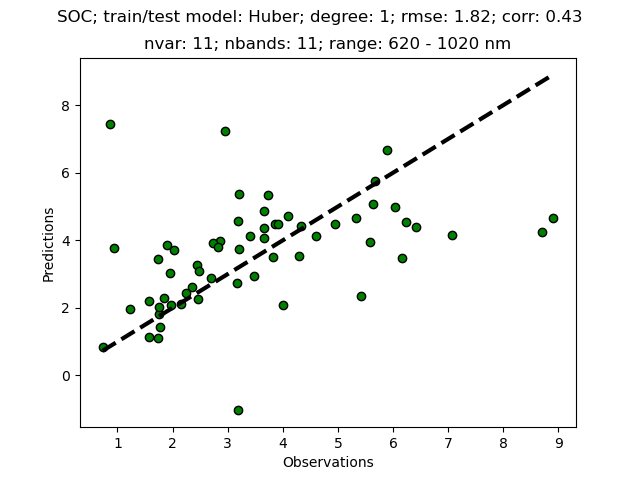
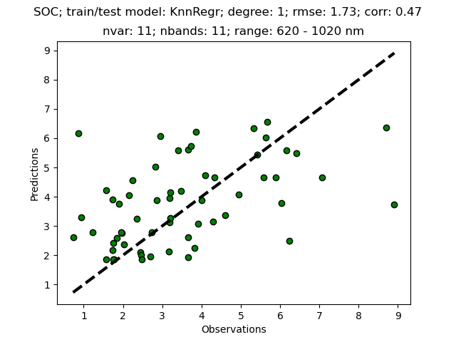
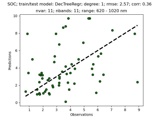
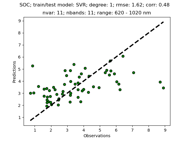
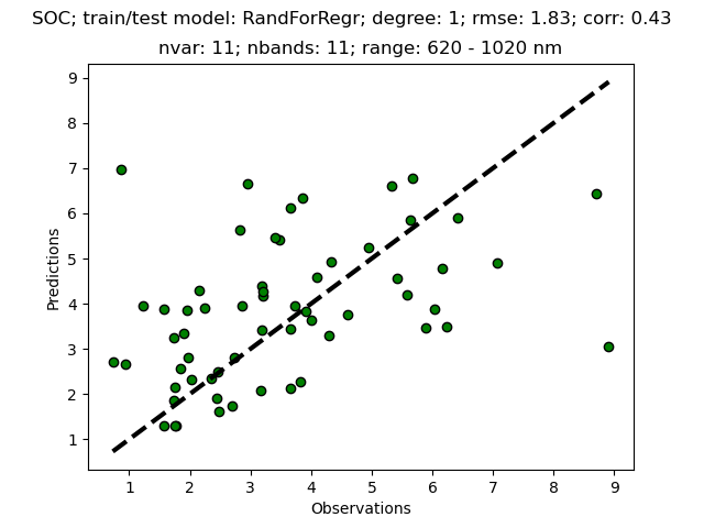
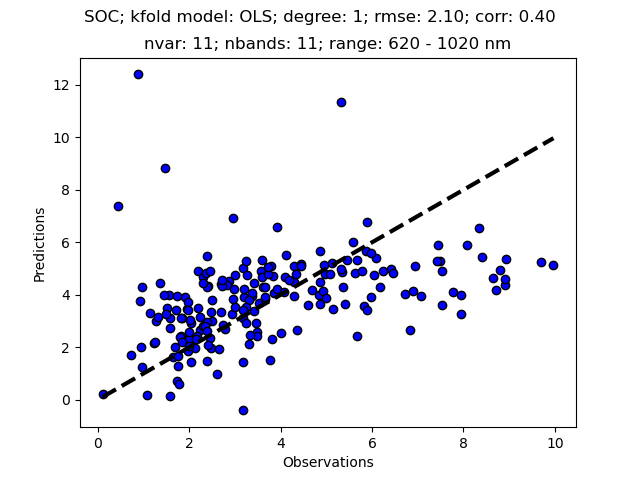
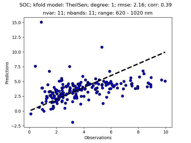
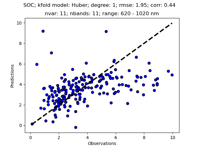
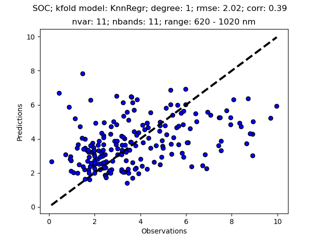
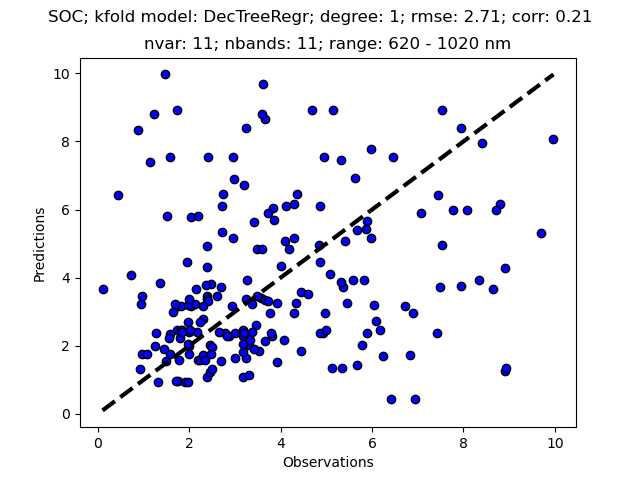
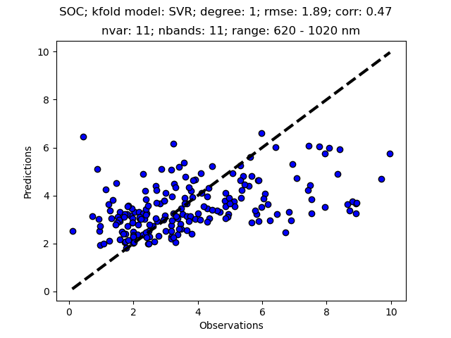
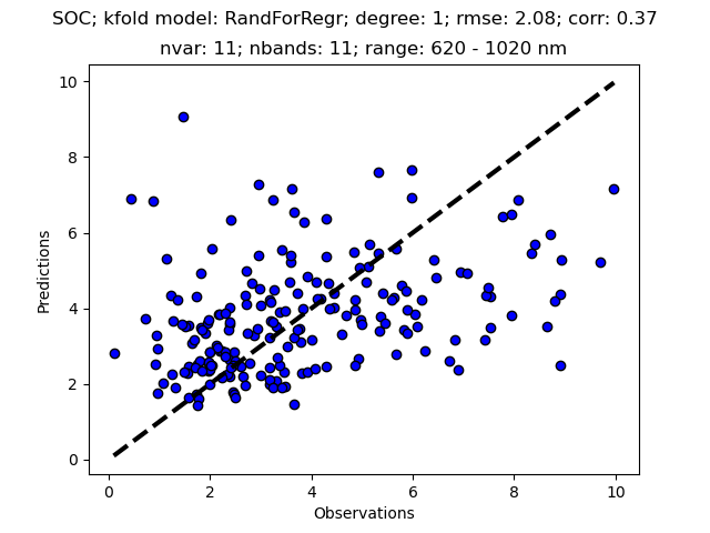
Soil Organic Carbon (SOC)

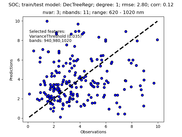
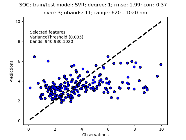
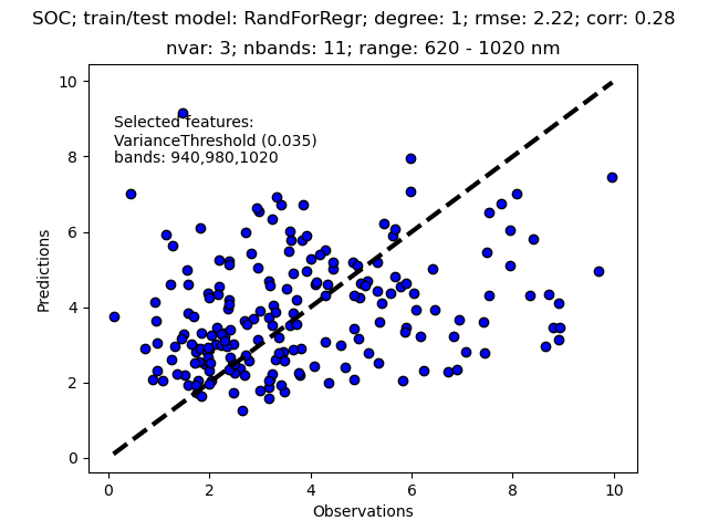
1 degree train/test

Comparison of train/test (0.7/0.3) SOC predictions from various regressors using 11 raw bands in the NIR region, 620 - 1020 nm.

1 degree kfold (n=10)

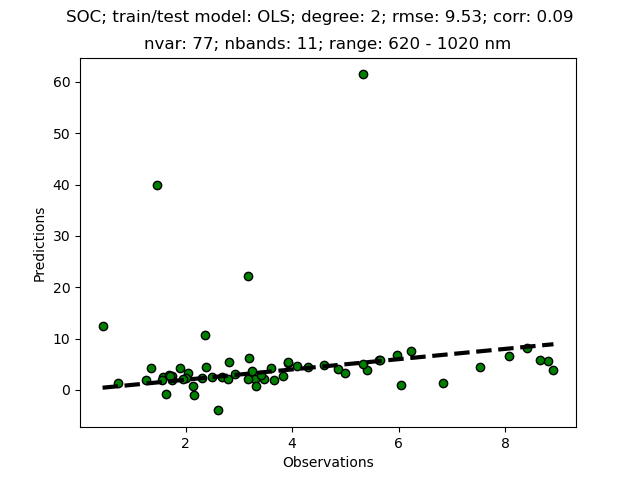
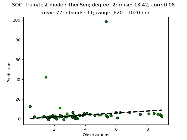
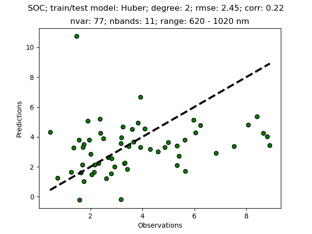
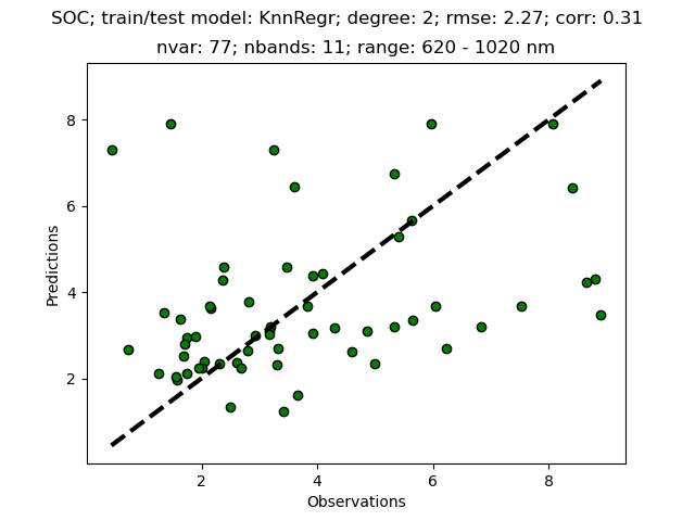
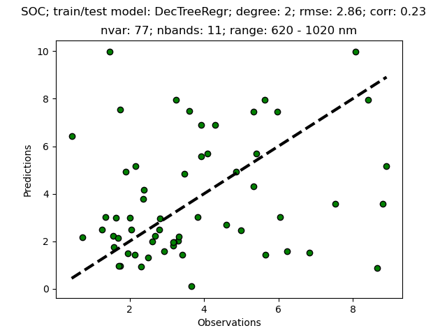
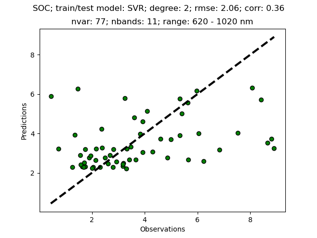
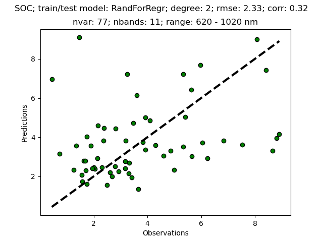
Comparison of kfold (n=10) SOC predictions from various regressors using 11 raw bands in the NIR region, 620 - 1020 nm.

2 degree train/test

The 2-degree models, created by using sklearn.preprocessing.PolynomialFeatures get 77 co-variables upon expansion of the origianl 11 bands. These models are thus massively overparameterised.

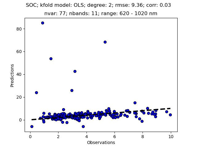
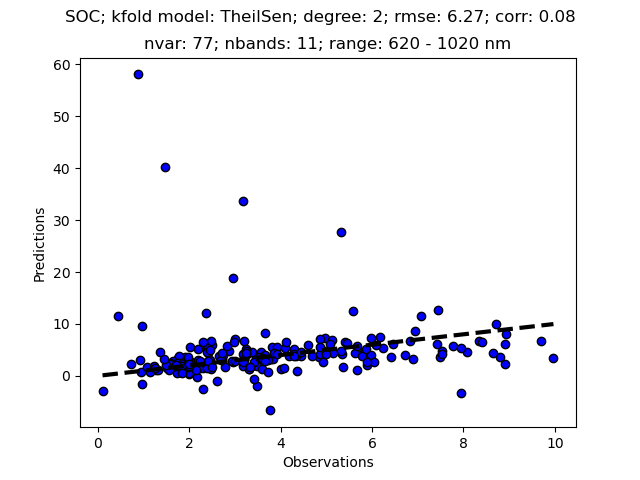
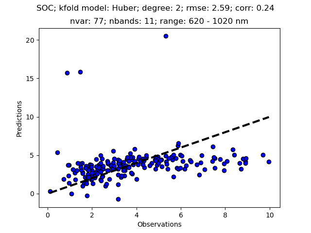
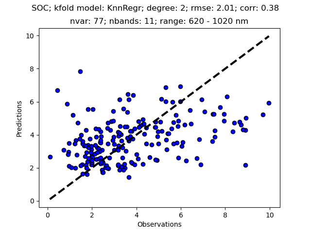
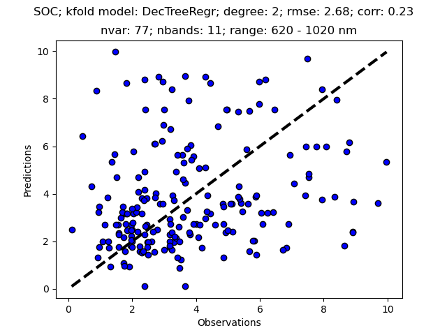
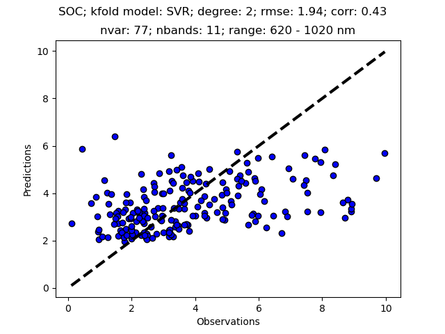
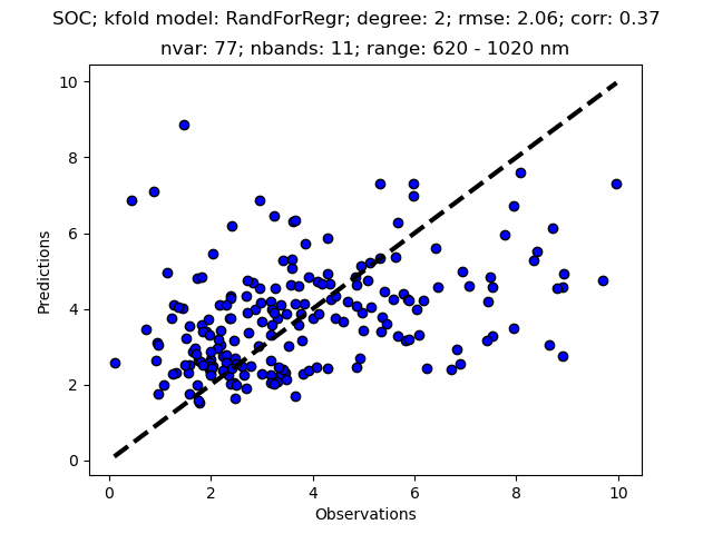
Comparison of train/test (0.7/0.3) SOC predictions from various regressors using an expanded polynomial of 77 covariates derived from 11 original bands in the NIR region, 620 - 1020 nm.

2 degree kfold

The 2-degree models, created by using sklearn.preprocessing.PolynomialFeatures get 77 co-variables upon expansion of the origianl 11 bands. These models are thus massively overparameterised.

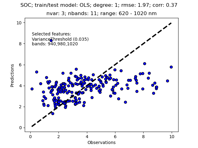
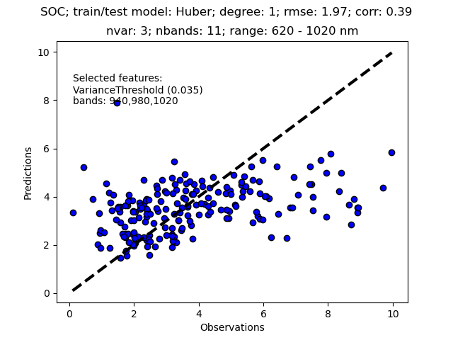
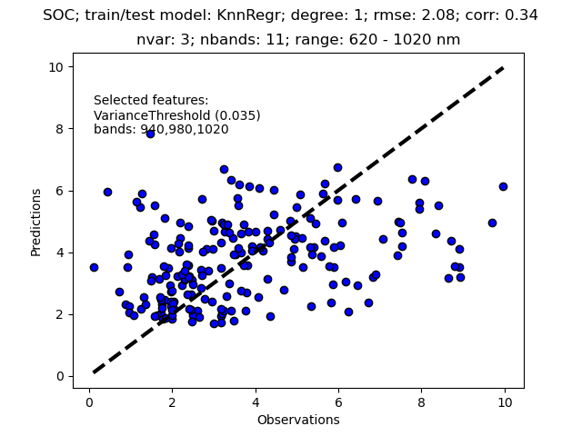
Comparison of kfold (n=10) SOC predictions from various regressors using an expanded polynomial of 77 covariates derived from 11 original bands in the NIR region, 620 - 1020 nm.

1 degree kfold with after feature selection

Using 11 consecutive bands probably causes overfitting as the bands are closely correlated. To reduce the number of covariates (bands) a simple method to use is to only retain those covariates that have a variance above a given threshold. In this example I have uses the variance threshold feature selection method and removed 8 bands and only retained the 3 bands with the highest variance for model development.

Comparison of kfold (n=10) SOC predictions from various regressors using 3 selected raw bands in the NIR region, 620 - 1020 nm.

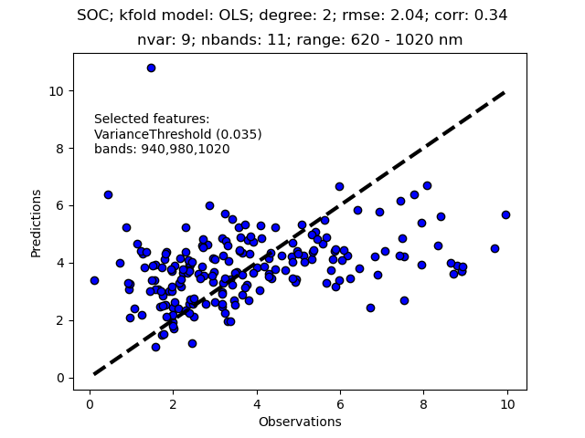
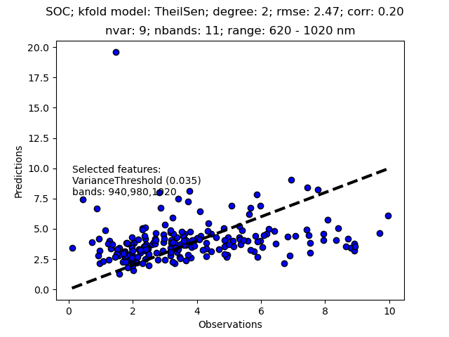
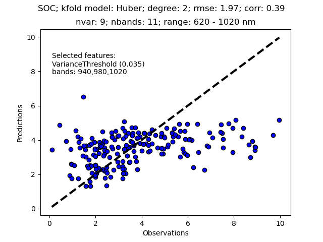
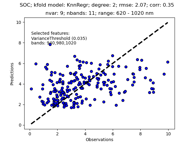
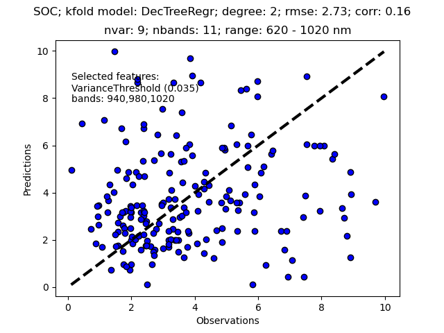
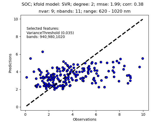
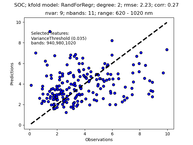
2 degree kfold with after feature selection

Comparison of kfold (n=10) SOC predictions from various regressors using polynomial expansions of 3 selected raw bands in the NIR region, 620 - 1020 nm.

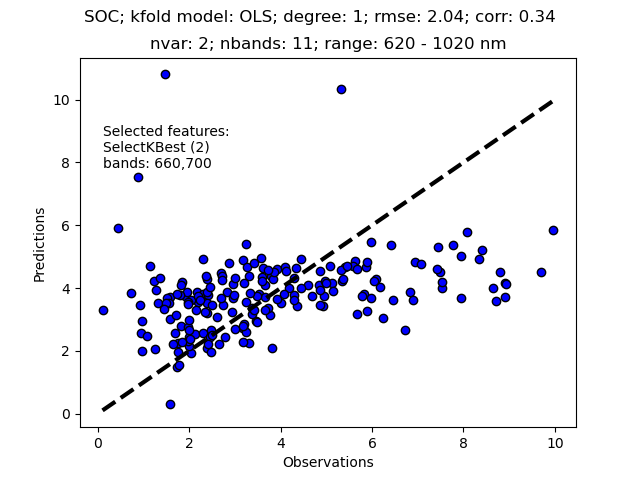
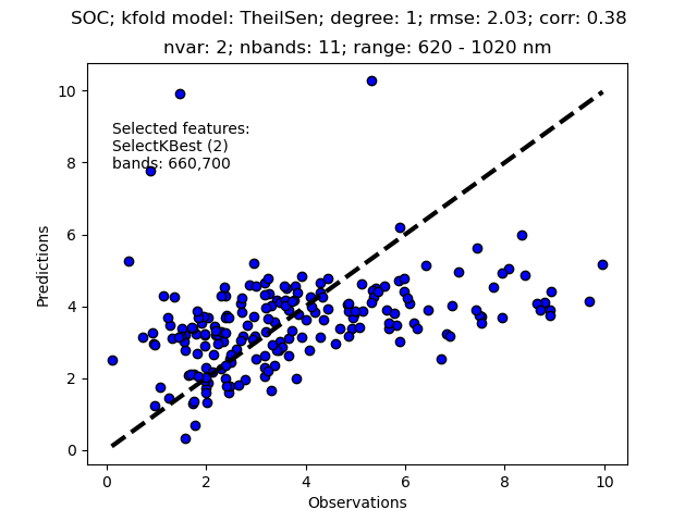
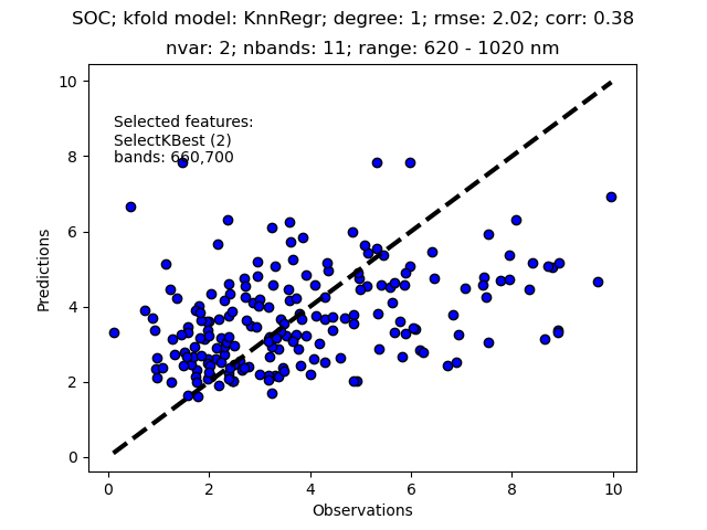
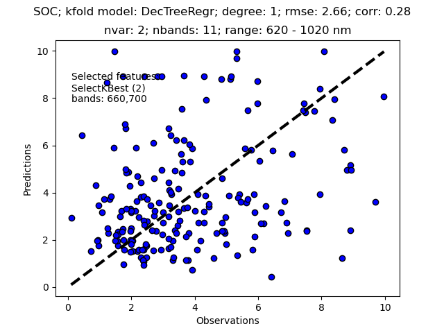
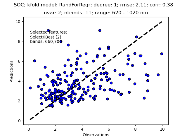
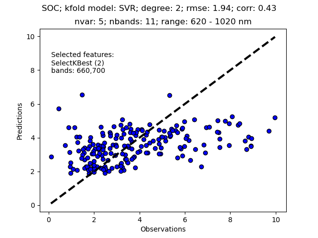
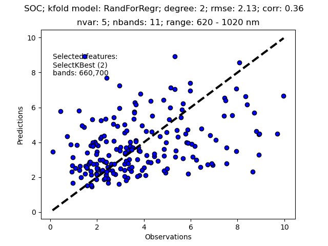
1 degree kfold with after KBest feature selection

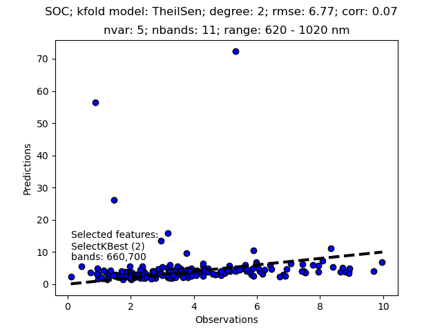
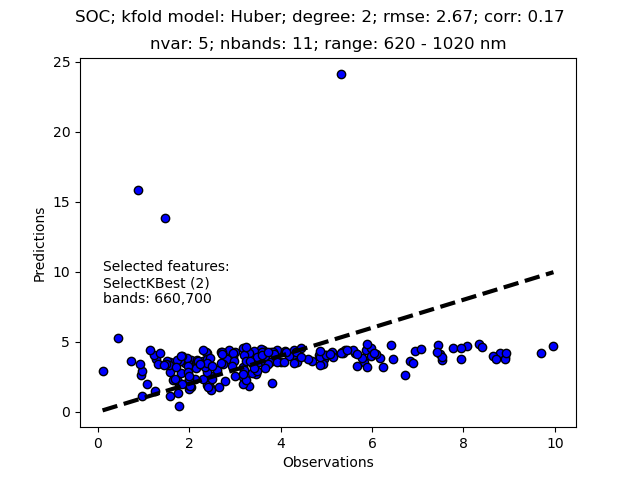
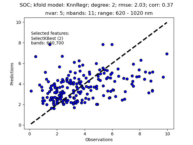
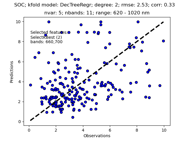
Here I have used KBest to retain the 2 bands with highest score. The retained bands (660 and 700 nm) differ from the bands with the highest variance (940, 980, and 1020 nm).

Comparison of kfold (n=10) SOC predictions from various regressors using 2 KBest selected raw bands in the NIR region, 620 - 1020 nm.

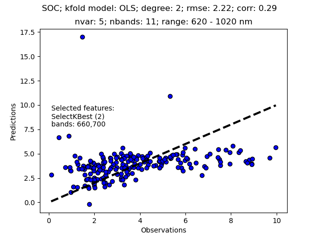
2 degree kfold with after KBest feature selection

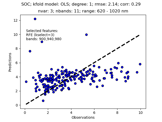
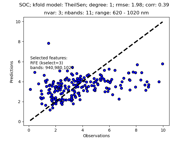
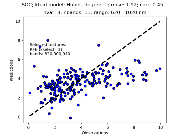
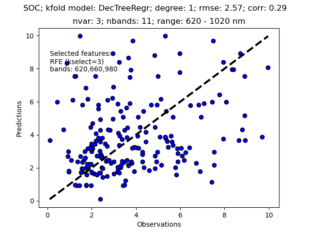
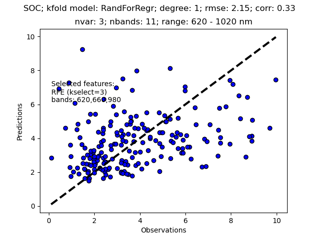
Comparison of kfold (n=10) SOC predictions from various regressors using 2 KBest selected raw bands with polynomial expansion to 5 covariates in the NIR region, 620 - 1020 nm.

1 degree kfold after RFE feature selection

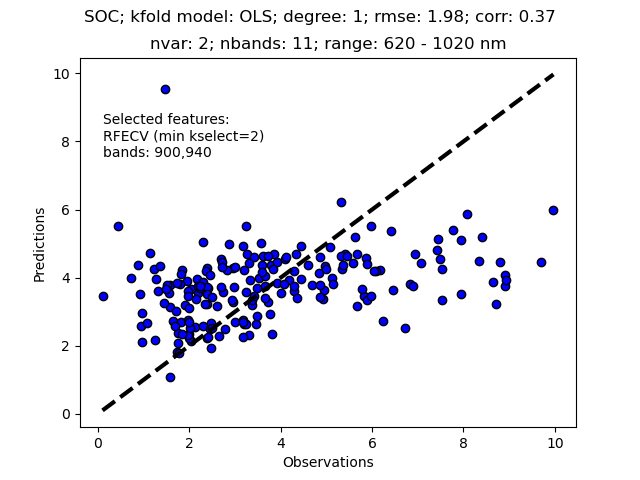
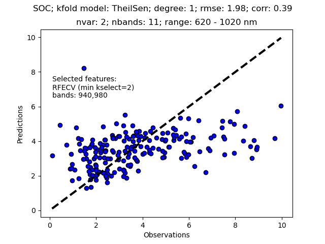
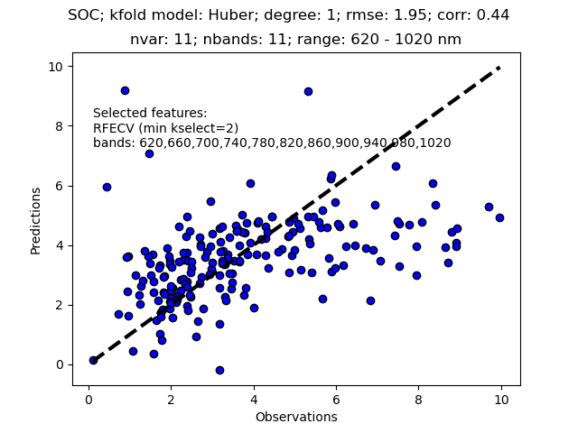
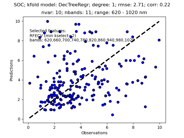
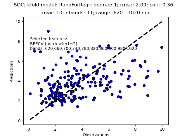
Comparison of kfold (n=10) SOC predictions from various regressors using 3 RFE selected raw bands in the NIR region, 620 - 1020 nm.

1 degree kfold after RFECV feature selection

RFECV inlcudes an internal function for selecting an optimal set of covariates. The selection depends on the model used and thus the nr of feature (covariates) varies.

Comparison of kfold (n=10) SOC predictions from various regressors using RFECV selection on model specifik raw bands in the NIR region, 620 - 1020 nm.

Resources

Polynomial Regression in Python using scikit-learn, by Tamas Ujhelyi.