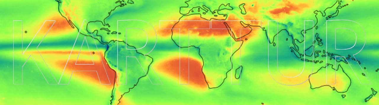
Introduction
Processing a global DEM all the way form downloading tiles to create coherent indices and metrics of landscapes, is a typical task for which Karttur’s GeoImagine Framework was built. Once the DEM is imported and organized within the Framework, it is easy to test different algorithms and visualizations for DEM. If you have access to some ground data you can also apply the Framework for comparing the results of different algorithms and parameters against ground data, and thus select the most appropriate landscape model.
Prerequisits
You must have installed Karttur’s GeoImagine Framework, and registered a user with a project that covers the geographic regions of the DEM you want to process.
Overview
This post summarises the processes chain for DEM data in Karttur’s GeoImagine Framework. Each step in the process chain is explained in more detail in linked posts.
A note on hydrological corrections
Before running the DEM processing you need to decide how you want to manage hydrological errors in your DEM. If there are no errors, then you do not need to worry, but usually there are at least both pits and flat area. Both of these problems primarily affects the extraction of river basins. Different algorithms handle these problems differently. The simplest solution is to fill up all pits completely, with or without tilting the flow across flat surfaces. This, however, causes the normally known relative DEM accuracy to be replaced by an unknown error that might, or might not, have spatial or contextual biases. If the DEM is going to be solely used for flow routing this is perhaps the best method. The alterantive is to to only fill up minor errors and errors that can be logically identied. The latter category would then include depressed channels and negative elevations along shorelines - and this is how it is done in this manual. But then you must also apply a flow routing algorithm that can pass depressions on the fly. The GRASS GIS module r.watershed does just that. And r.watershed is used for the DEM modelling in this post. To fill up all depressions, you can instead use the GRASS GIS module r.terraflow, or any of the DEM filling algorithms of SAGA GIS. If you apply hydrological DEM corrections, you must also decide which DEM aleternative (corrected or non-corrected) to use for ectracting other indexes, like slope, curvature etc.
Process chain
The process chain is available at Kartturs GitHub account and also found under the Hide/show button below. The process chain is an ordinary text file linking to a series of json files. Empty rows and rows starting with a “#” are ignored. When called from karttur’s GeoImagine Framework, the processes of each json file are sequentially run. The structure of the json files and the commands are summarised in the post [#]#().
###################################
###################################
###      Copernicus DEM         ###
###################################
###################################

###################################
###           Layout            ###
###################################

## json/0001_CreatesScaling_DEM_v090.json

## json/0002_AddRasterPalette_DEM_v090.json

## json/0003_createlegends_DEM_v090.json

## json/0005_exportlegend_DEM_v090.json

###################################
###     Search and download     ###
###################################

## json/0100_SearchCopernicusProducts_CopDEM-90m.json

## json/0110_DownloadCopernicus_CopDEM-90m.json

###################################
###            UnZip            ###
###################################

## json/0120_UnZipRawData_CopDEM-90m.json

###################################
###       Mosaic Download       ###
###################################

## json/0125_MosaicAncillary_CopDEM-90m.json

## json/0125-COPDEM30-mosaic-raw.json

###################################
###           Organize          ###
###################################

## json/0160-Ancillary-import-CopDEM90.json

## json/0160-Ancillary-import-CopDEM30.json

###################################
###            Tiling           ###
###################################

## json/0180_TileAncillaryRegion_CopDem-30m.json

## json/0180_TileAncillaryRegion_CopDem-90m.json

###################################
###         Mosaic tiles        ###
###################################

## json/0190_MosaicAdjacentTiles_CopDEM-30m.json

## json/0190_MosaicAdjacentTiles_CopDEM-90m.json

###################################
###       DEM Corrections       ###
###################################

## Fill single pits and peaks (adjacent to streams)
## json/0230_GrassDemFillDirTiles_CopDEM_90m.json

## Create virtual mosaics of the filled DEM
## json/0191_MosaicAdjacentTiles_CopDEM-90m.json

## Fill larger pits in streams with r.hydrodem
## json/0240_GrassDemHydroDemTiles_CopDEM-90m.json

## Create virtual mosaics of the twice filled DEM
## json/0192_MosaicAdjacentTiles_CopDEM-90m.json

#############################################
### River mouth and Shoreline corrections ###
#############################################

## json/0210_GrassOnetoManyTiles-correct-shoreline_CopDEM-90m.json

###################################
###  DEM kernel based derivates ###
###################################

## json/0301_GdalDemTiles_CopDEM-90m.json

## ?? json/0310_CopernicusDEM_gdaldem_ease2n.json

## json/0303_NumpyDemTiles_CopDEM-90m.json

## ?? json/0312_COPDEM_numpydemtpi_ease2n.json

## ?? json/0310_CopDEM_grassdem_ease2n.json

## Create DEM derivates at 3x3 and 9x9 cells
## /json/0305_GrassOnetoManyTiles-DEM-derivates-3+9cell_CopDEM-90m.json

###################################
###   DEM hillslope derivates   ###
###################################

## json/0311_GrassOnetoManyTiles_hillslope-derivates_copDEM-90m.json

###################################
###     DEM basin extraction    ###
###################################

## json/0321_GrassOnetoManyTilesCopDEM-basin-extract-stage2_copDEM.json
## json/0321b_GrassOnetoManyTilesCopDEM-basin-extract-stage2_copDEM.json

## After 0321_GrassOnetoManyTilesCopDEM-basin-## extract-stage2_copDEM
## json/0325_BasinOutletTiles_CopDEM-90m.json

# Extra output from the grass session above

## json/0315_CopDEM_Basin-outlets-tiles-r-out-gdal_ease2n.json

###################################
###     Define hydro regions    ###
###################################

## Reduce resolution to 1 km
## NOT REQUIRED
## json/0313_CopDEM_translate1km_ease2n.json

## Mosaic entire northern hemisphere at 90m
## json/0313_CopDEM_mosaic1km_ease2n.json

###################################
###   Mosaic to Hydro regions   ###
###################################

## json/0225_MosaicTiles-copDEM.json

###################################
###       Extract raster        ###
###################################

## WORKINPROGRESS ExtractTilesPointList

###################################
###        Export tiles         ###
###################################

### Export elevation data with different color ramps
## json/0905A_ExportTilesToByte_CopDEM-elevation_v090.json

### Export shaded elevation data with different color ramps
## json/0906A_ExportShadedTilesToByte_CopDEM-elevation_v090.json

## json/0905_DEM-curvature_ExportShadeTilesToByte_v090.json

## json/0905_DEM_ExportTilesToByte_v090.json

## json/0905_DEM-slope_ExportTilesToByte_v090.json

## json/0905_DEM-TRI_ExportTilesToByte_v090.json

#json/0905_DEM-landforms_ExportTilesToByte_v090.json

## json/0905_DEM_ExportShadeTilesToByte_v090.json

## json/0905_terrain_ExportTilesToByte_v090.json

## json/0906_DEM-elevation_ExportShadeTilesToByte_v090.json

## json/0906_DEM-curvature_ExportShadeTilesToByte_v090.json

###################################
###       Duplicate tiles       ###
###################################

json/0950_duplicate_CopDEM_v090.json

###################################
###        Archive tiles        ###
###################################

## json/0960b_ZipArchive_DEM_v090.json
Layout
To produce symbolised and labeled map using the Framework, you have to define some Layout features and parameters. All map layout is done using unsigned byte range maps with values ranging from 1 to 255, Where values 251 to 255 are reserved for specific purposes and not allowed for representing map values. To produce a symbolised map using the Framework you need to define the scaling and the palette.
Layout processes include:
- CreateScaling,
- AddRasterPalette,
- CreateLegend, and
- ExportLegend.
CreateScaling
json/0001_CreatesScaling_DEM_v090.json
The CreateScaling process converts any input raster into an unsigned byte (0-255) range file. The byte file is then used for assigning a color ramp (defined by the process AddRasterPalette, see next section).
Scaling is thus not defined on the fly, instead each map composition (see the post on ??? for an explanation on the Framework map composition concept) must be associated with a predefined scaling. Once defined, this scaling can not be changed.
{
  "userproject": {
    "userid": "karttur",
    "projectid": "karttur",
    "tractid": "karttur",
    "siteid": "*",
    "plotid": "*",
    "system": "system"
  },
  "period": {
    "timestep": "static"
  },
  "process": [
    {
      "processid": "CreateScaling",
      "overwrite": false,
      "parameters": {
        "scalefac": 0.03125,
        "mirror0": false
      },
      "comp": [
        {
          "dem": {
            "source": "*",
            "product": "*",
            "content": "dem",
            "layerid": "dem",
            "suffix": "*"
          }
        }
      ]
    },
    {
      "processid": "CreateScaling",
      "overwrite": false,
      "parameters": {
        "scalefac": 1,
        "mirror0": false
      },
      "comp": [
        {
          "dem": {
            "source": "*",
            "product": "*",
            "content": "dem",
            "layerid": "dem1",
            "suffix": "*"
          }
        }
      ]
    },
    {
      "processid": "CreateScaling",
      "overwrite": false,
      "parameters": {
        "scalefac": 4,
        "mirror0": false
      },
      "comp": [
        {
          "slope": {
            "source": "*",
            "product": "*",
            "content": "dem",
            "layerid": "slope",
            "suffix": "*"
          }
        }
      ]
    },
    {
      "processid": "CreateScaling",
      "overwrite": false,
      "parameters": {
        "scalefac": 1,
        "mirror0": true
      },
      "comp": [
        {
          "shade": {
            "source": "*",
            "product": "*",
            "content": "dem",
            "layerid": "shade",
            "suffix": "*"
          }
        }
      ]
    },
    {
      "processid": "CreateScaling",
      "overwrite": true,
      "parameters": {
        "scalefac": 5,
        "mirror0": true
      },
      "comp": [
        {
          "tpi": {
            "source": "*",
            "product": "*",
            "content": "dem",
            "layerid": "tpi",
            "suffix": "*"
          }
        }
      ]
    },
    {
      "processid": "CreateScaling",
      "overwrite": true,
      "parameters": {
        "scalefac": 5,
        "mirror0": false
      },
      "comp": [
        {
          "tri": {
            "source": "*",
            "product": "*",
            "content": "dem",
            "layerid": "tri",
            "suffix": "*"
          }
        }
      ]
    },
    {
      "processid": "CreateScaling",
      "overwrite": false,
      "parameters": {
        "scalefac": 50000,
        "mirror0": true
      },
      "comp": [
        {
          "profc": {
            "source": "*",
            "product": "*",
            "content": "dem",
            "layerid": "profc",
            "suffix": "*"
          }
        },
        {
          "crosc": {
            "source": "*",
            "product": "*",
            "content": "dem",
            "layerid": "crosc",
            "suffix": "*"
          }
        },
        {
          "longc": {
            "source": "*",
            "product": "*",
            "content": "dem",
            "layerid": "longc",
            "suffix": "*"
          }
        }
      ]
    },
    {
      "processid": "CreateScaling",
      "overwrite": false,
      "parameters": {
        "scalefac": 1000,
        "mirror0": true
      },
      "comp": [
        {
          "planc": {
            "source": "*",
            "product": "*",
            "content": "dem",
            "layerid": "planc",
            "suffix": "*"
          }
        }
      ]
    },
    {
      "processid": "CreateScaling",
      "overwrite": false,
      "parameters": {
        "scalefac": 25,
        "mirror0": false
      },
      "comp": [
        {
          "rusle-slopelength": {
            "source": "*",
            "product": "*",
            "content": "terrain",
            "layerid": "rusle-slopelength",
            "suffix": "*"
          }
        }
      ]
    },
    {
      "processid": "CreateScaling",
      "overwrite": false,
      "parameters": {
        "scalefac": 50,
        "offsetadd": -2,
        "mirror0": false
      },
      "comp": [
        {
          "rusle-slopesteepness": {
            "source": "*",
            "product": "*",
            "content": "terrain",
            "layerid": "rusle-slopesteepness",
            "suffix": "*"
          }
        }
      ]
    },
    {
      "processid": "CreateScaling",
      "overwrite": false,
      "parameters": {
        "scalefac": 2,
        "offsetadd": 25,
        "mirror0": false
      },
      "comp": [
        {
          "near-divide-head": {
            "source": "*",
            "product": "*",
            "content": "terrain",
            "layerid": "near-divide-head",
            "suffix": "*"
          }
        }
      ]
    },
    {
      "processid": "CreateScaling",
      "overwrite": false,
      "parameters": {
        "scalefac": 2,
        "offsetadd": 25,
        "mirror0": false
      },
      "comp": [
        {
          "far-divide-head": {
            "source": "*",
            "product": "*",
            "content": "terrain",
            "layerid": "far-divide-head",
            "suffix": "*"
          }
        }
      ]
    },
    {
      "processid": "CreateScaling",
      "overwrite": false,
      "parameters": {
        "scalefac": 2,
        "offsetadd": 25,
        "mirror0": false
      },
      "comp": [
        {
          "near-divide-head": {
            "source": "*",
            "product": "*",
            "content": "terrain",
            "layerid": "near-divide-head",
            "suffix": "*"
          },
          "far-divide-head": {
            "source": "*",
            "product": "*",
            "content": "terrain",
            "layerid": "far-divide-head",
            "suffix": "*"
          },
          "hydraulhead": {
            "source": "*",
            "product": "*",
            "content": "terrain",
            "layerid": "hydraulhead",
            "suffix": "*"
          }
        }
      ]
    },
    {
      "processid": "CreateScaling",
      "overwrite": false,
      "parameters": {
        "scalefac": 0.05555,
        "mirror0": false
      },
      "comp": [
        {
          "stream-dist": {
            "source": "*",
            "product": "*",
            "content": "terrain",
            "layerid": "stream-dist",
            "suffix": "v01-pfpf-hydrdem4+4-90m"
          }
        }
      ]
    },
    {
      "processid": "CreateScaling",
      "overwrite": false,
      "parameters": {
        "scalefac": 0.1111,
        "mirror0": false
      },
      "comp": [
        {
          "near-divide-dist": {
            "source": "*",
            "product": "*",
            "content": "terrain",
            "layerid": "near-divide-dist",
            "suffix": "v01-pfpf-hydrdem4+4-90m"
          }
        }
      ]
    },
    {
      "processid": "CreateScaling",
      "overwrite": false,
      "parameters": {
        "scalefac": 0.01111,
        "mirror0": false
      },
      "comp": [
        {
          "far-divide-dist": {
            "source": "*",
            "product": "*",
            "content": "terrain",
            "layerid": "far-divide-dist",
            "suffix": "v01-pfpf-hydrdem4+4-90m"
          }
        }
      ]
    },
    {
      "processid": "CreateScaling",
      "overwrite": false,
      "parameters": {
        "scalefac": 12,
        "log": true,
        "mirror0": false
      },
      "comp": [
        {
          "sfd-updrain": {
            "source": "*",
            "product": "*",
            "content": "terrain",
            "layerid": "sfd-updrain",
            "suffix": "*"
          }
        }
      ]
    },
    {
      "processid": "CreateScaling",
      "overwrite": false,
      "parameters": {
        "scalefac": 12,
        "log": true,
        "mirror0": false
      },
      "comp": [
        {
          "mfd-updrain": {
            "source": "*",
            "product": "*",
            "content": "terrain",
            "layerid": "mfd-updrain",
            "suffix": "*"
          }
        }
      ]
    },
    {
      "processid": "CreateScaling",
      "overwrite": false,
      "parameters": {
        "scalefac": 20,
        "log": true,
        "mirror0": false
      },
      "comp": [
        {
          "psi": {
            "source": "*",
            "product": "*",
            "content": "terrain",
            "layerid": "psi",
            "suffix": "*"
          }
        }
      ]
    },
    {
      "processid": "CreateScaling",
      "overwrite": false,
      "parameters": {
        "scalefac": 20,
        "log": true,
        "mirror0": false
      },
      "comp": [
        {
          "spi": {
            "source": "*",
            "product": "*",
            "content": "terrain",
            "layerid": "spi",
            "suffix": "*"
          }
        }
      ]
    },
    {
      "processid": "CreateScaling",
      "overwrite": false,
      "parameters": {
        "scalefac": 10,
        "offsetadd": -30,
        "mirror0": false
      },
      "comp": [
        {
          "tci": {
            "source": "*",
            "product": "*",
            "content": "terrain",
            "layerid": "tci",
            "suffix": "*"
          }
        }
      ]
    },
    {
      "processid": "CreateScaling",
      "overwrite": false,
      "parameters": {
        "scalefac": 1,
        "mirror0": false
      },
      "comp": [
        {
          "lftpi": {
            "source": "*",
            "product": "*",
            "content": "dem",
            "layerid": "landform-tpi",
            "suffix": "*"
          }
        },
        {
          "landform-ps": {
            "source": "*",
            "product": "*",
            "content": "dem",
            "layerid": "landform-ps",
            "suffix": "*"
          }
        }
      ]
    },
    {
      "processid": "CreateScaling",
      "overwrite": true,
      "parameters": {
        "scalefac": 10,
        "mirror0": false
      },
      "comp": [
        {
          "lfgeomrph": {
            "source": "*",
            "product": "*",
            "content": "dem",
            "layerid": "geomorph",
            "suffix": "*"
          }
        }
      ]
    },
    {
      "processid": "CreateScaling",
      "overwrite": true,
      "parameters": {
        "scalefac": 10,
        "mirror0": false
      },
      "comp": [
        {
          "landform-ps": {
            "source": "*",
            "product": "*",
            "content": "dem",
            "layerid": "landform-ps",
            "suffix": "*"
          }
        }
      ]
    }
  ]
}
AddRasterPalette
json/0002_AddRasterPalette_DEM_v090.json
In contrast to the scaling, the palette can be freely set for any map composition (but using the same scaling). The palette to use for any map layout is defined when calling the process that generates the layout.
{
"userproject": {
"userid": "karttur",
"projectid": "karttur",
"tractid": "karttur",
"siteid": "*",
"plotid": "*",
"system": "system"
},
"period": {
"timestep": "static"
},
"process": [
{
"processid": "AddRasterPalette",
"overwrite": true,
"parameters": {
"palette": "dem_dark_auto",
"compid": "dem_dark_auto",
"setcolor": {
"0": {
"red": "54",
"green": "121",
"blue": "36",
"alpha": "0",
"label": "auto",
"hint": "auto"
},
"125": {
"red": "247",
"green": "248",
"blue": "80",
"alpha": "0",
"label": "auto",
"hint": "auto"
},
"250": {
"red": "121",
"green": "24",
"blue": "21",
"alpha": "0",
"label": "auto",
"hint": "auto"
},
"251": {
"red": "0",
"green": "0",
"blue": "0",
"alpha": "0",
"label": "upland drainage",
"hint": "upland drainage"
},
"255": {
"red": "0",
"green": "0",
"blue": "0",
"alpha": "0",
"label": "upland drainage",
"hint": "upland drainage"
}
}
}
},
{
"processid": "AddRasterPalette",
"overwrite": true,
"parameters": {
"palette": "landformTPI",
"compid": "dem_landform-TPI",
"setcolor": {
"5": {
"red": "30",
"green": "0",
"blue": "170",
"alpha": "0",
"label": "Canyon or valley",
"hint": "NA"
},
"12": {
"red": "30",
"green": "0",
"blue": "170",
"alpha": "0",
"label": "Canyon or valley",
"hint": "Canyon or valley"
},
"13": {
"red": "10",
"green": "160",
"blue": "10",
"alpha": "0",
"label": "midslope/shallow valley, hollow",
"hint": "NA"
},
"22": {
"red": "10",
"green": "160",
"blue": "10",
"alpha": "0",
"label": "midslope/shallow valley, hollow",
"hint": "midslope/shallow valley, hollow"
},
"23": {
"red": "25",
"green": "155",
"blue": "234",
"alpha": "0",
"label": "upland drainage",
"hint": "NA"
},
"32": {
"red": "25",
"green": "155",
"blue": "234",
"alpha": "0",
"label": "upland drainage",
"hint": "upland drainage"
},
"33": {
"red": "0",
"green": "128",
"blue": "128",
"alpha": "0",
"label": "U-shaped valley or footslope",
"hint": "NA"
},
"42": {
"red": "0",
"green": "128",
"blue": "128",
"alpha": "0",
"label": "U-shaped valley or footslope",
"hint": "U-shaped valley or footslope"
},
"43": {
"red": "220",
"green": "235",
"blue": "240",
"alpha": "0",
"label": "plain",
"hint": "NA"
},
"52": {
"red": "220",
"green": "235",
"blue": "240",
"alpha": "0",
"label": "plain",
"hint": "plain or flat"
},
"53": {
"red": "230",
"green": "230",
"blue": "120",
"alpha": "0",
"label": "open slope",
"hint": "NA"
},
"62": {
"red": "230",
"green": "230",
"blue": "120",
"alpha": "0",
"label": "open slope",
"hint": "open slope"
},
"63": {
"red": "235",
"green": "205",
"blue": "15",
"alpha": "0",
"label": "upper slope",
"hint": "NA"
},
"72": {
"red": "235",
"green": "205",
"blue": "15",
"alpha": "0",
"label": "upper slope",
"hint": "mesa, upper slope, shoulder, ridge"
},
"73": {
"red": "255",
"green": "128",
"blue": "10",
"alpha": "0",
"label": "local ridge",
"hint": "NA"
},
"82": {
"red": "255",
"green": "128",
"blue": "10",
"alpha": "0",
"label": "local ridge",
"hint": "lodal ridge"
},
"83": {
"red": "224",
"green": "80",
"blue": "80",
"alpha": "0",
"label": "midslope ridge or spur",
"hint": "NA"
},
"92": {
"red": "224",
"green": "80",
"blue": "80",
"alpha": "0",
"label": "midslope ridge or spur",
"hint": "midslope ridge or spur"
},
"93": {
"red": "180",
"green": "20",
"blue": "10",
"alpha": "0",
"label": "peak",
"hint": "NA"
},
"102": {
"red": "180",
"green": "20",
"blue": "10",
"alpha": "0",
"label": "peak",
"hint": "peak or summit"
},
"107": {
"red": "180",
"green": "20",
"blue": "10",
"alpha": "0",
"label": "peak",
"hint": "NA"
},
"255": {
"red": "0",
"green": "0",
"blue": "0",
"alpha": "255",
"label": "255",
"hint": "no data"
}
}
}
},
{
"processid": "AddRasterPalette",
"overwrite": true,
"parameters": {
"palette": "landformTPIdouble",
"compid": "landform-TPIx",
"setcolor": {
"11": {
"red": "0",
"green": "0",
"blue": "200",
"alpha": "0",
"label": "Canyon or valley",
"hint": "Canyon or valley"
},
"12": {
"red": "55",
"green": "0",
"blue": "150",
"alpha": "0",
"label": "Canyon or valley",
"hint": "Canyon or valley"
},
"21": {
"red": "0",
"green": "200",
"blue": "0",
"alpha": "0",
"label": "shallow valley",
"hint": "shallow valley or hollow"
},
"22": {
"red": "0",
"green": "180",
"blue": "135",
"alpha": "0",
"label": "midslope drainage",
"hint": " midslope drainage or shallow valley or hollow"
},
"31": {
"red": "50",
"green": "50",
"blue": "200",
"alpha": "0",
"label": "upland drainage",
"hint": "upland drainage"
},
"32": {
"red": "25",
"green": "25",
"blue": "225",
"alpha": "0",
"label": "upland drainage",
"hint": "upland drainage"
},
"41": {
"red": "0",
"green": "155",
"blue": "244",
"alpha": "0",
"label": "U-shaped valley",
"hint": "U-shaped valley or footslope"
},
"42": {
"red": "0",
"green": "100",
"blue": "200",
"alpha": "0",
"label": "Footslope",
"hint": "U-shaped valley or footslope"
},
"50": {
"red": "220",
"green": "220",
"blue": "220",
"alpha": "0",
"label": "plain",
"hint": "plain or flat"
},
"60": {
"red": "251",
"green": "255",
"blue": "0",
"alpha": "0",
"label": "open slope",
"hint": "open slope"
},
"71": {
"red": "255",
"green": "56",
"blue": "0",
"alpha": "0",
"label": "upper slope",
"hint": "upper slope, shoulder, ridge"
},
"72": {
"red": "130",
"green": "130",
"blue": "0",
"alpha": "0",
"label": "mesa",
"hint": "mesa, upper slope, shoulder, ridge"
},
"81": {
"red": "255",
"green": "213",
"blue": "112",
"alpha": "0",
"label": "local ridge",
"hint": "lodal ridge (midslope)"
},
"82": {
"red": "255",
"green": "213",
"blue": "112",
"alpha": "0",
"label": "local ridge",
"hint": "local ridge (in plain)"
},
"91": {
"red": "254",
"green": "214",
"blue": "0",
"alpha": "0",
"label": "midslope ridge or spur",
"hint": "midslope ridge or spur"
},
"92": {
"red": "254",
"green": "214",
"blue": "0",
"alpha": "0",
"label": "midslope ridge or spur",
"hint": "midslope ridge or spur"
},
"101": {
"red": "140",
"green": "0",
"blue": "0",
"alpha": "0",
"label": "peak",
"hint": "peak or summit"
},
"102": {
"red": "100",
"green": "0",
"blue": "0",
"alpha": "0",
"label": "peak",
"hint": "peak or summit"
},
"255": {
"red": "0",
"green": "0",
"blue": "0",
"alpha": "255",
"label": "255",
"hint": "no data"
}
}
}
},
{
"processid": "AddRasterPalette",
"overwrite": true,
"parameters": {
"palette": "slope",
"compid": "dem_slope",
"setcolor": {
"0": {
"red": "0",
"green": "92",
"blue": "128",
"alpha": "0",
"label": "0",
"hint": "slope = 0 (flat)"
},
"4": {
"red": "0",
"green": "128",
"blue": "64",
"alpha": "0",
"label": "1.0",
"hint": "NA"
},
"40": {
"red": "220",
"green": "240",
"blue": "16",
"alpha": "0",
"label": "10",
"hint": "slope = 10"
},
"80": {
"red": "255",
"green": "146",
"blue": "18",
"alpha": "0",
"label": "30",
"hint": "slope = 30"
},
"160": {
"red": "192",
"green": "46",
"blue": "0",
"alpha": "0",
"label": "50",
"hint": "slope = 50"
},
"250": {
"red": "128",
"green": "0",
"blue": "0",
"alpha": "0",
"label": "> 60",
"hint": "slope > 60"
},
"251": {
"red": "0",
"green": "0",
"blue": "0",
"alpha": "0",
"label": "upland drainage",
"hint": "upland drainage"
},
"255": {
"red": "0",
"green": "0",
"blue": "0",
"alpha": "0",
"label": "upland drainage",
"hint": "upland drainage"
}
}
}
},
{
"processid": "AddRasterPalette",
"overwrite": true,
"parameters": {
"palette": "slope2",
"compid": "dem_slope2",
"setcolor": {
"0": {
"red": "143",
"green": "152",
"blue": "18",
"alpha": "0",
"label": "0",
"hint": "slope = 0 (flat)"
},
"4": {
"red": "150",
"green": "160",
"blue": "33",
"alpha": "0",
"label": "1.0",
"hint": "NA"
},
"40": {
"red": "225",
"green": "240",
"blue": "51",
"alpha": "0",
"label": "10",
"hint": "slope = 10"
},
"80": {
"red": "255",
"green": "200",
"blue": "10",
"alpha": "0",
"label": "20",
"hint": "slope = 20"
},
"120": {
"red": "250",
"green": "160",
"blue": "40",
"alpha": "0",
"label": "30",
"hint": "slope = 30"
},
"160": {
"red": "245",
"green": "100",
"blue": "20",
"alpha": "0",
"label": "40",
"hint": "slope = 40"
},
"200": {
"red": "205",
"green": "70",
"blue": "120",
"alpha": "0",
"label": "50",
"hint": "slope = 50"
},
"250": {
"red": "179",
"green": "107",
"blue": "209",
"alpha": "0",
"label": "> 60",
"hint": "slope > 60"
},
"251": {
"red": "0",
"green": "0",
"blue": "0",
"alpha": "0",
"label": "upland drainage",
"hint": "upland drainage"
},
"255": {
"red": "0",
"green": "0",
"blue": "0",
"alpha": "0",
"label": "upland drainage",
"hint": "upland drainage"
}
}
}
},
{
"processid": "AddRasterPalette",
"overwrite": true,
"parameters": {
"palette": "slope3",
"compid": "dem_slope3",
"setcolor": {
"0": {
"red": "135",
"green": "160",
"blue": "212",
"alpha": "0",
"label": "0",
"hint": "slope = 0 (flat)"
},
"4": {
"red": "168",
"green": "179",
"blue": "149",
"alpha": "0",
"label": "1.0",
"hint": "NA"
},
"40": {
"red": "213",
"green": "222",
"blue": "115",
"alpha": "0",
"label": "10",
"hint": "slope = 10"
},
"80": {
"red": "253",
"green": "253",
"blue": "155",
"alpha": "0",
"label": "20",
"hint": "slope = 20"
},
"120": {
"red": "239",
"green": "184",
"blue": "12",
"alpha": "0",
"label": "30",
"hint": "slope = 30"
},
"160": {
"red": "223",
"green": "144",
"blue": "88",
"alpha": "0",
"label": "40",
"hint": "slope = 40"
},
"200": {
"red": "233",
"green": "129",
"blue": "189",
"alpha": "0",
"label": "50",
"hint": "slope = 50"
},
"250": {
"red": "216",
"green": "153",
"blue": "243",
"alpha": "0",
"label": "> 60",
"hint": "slope > 60"
},
"251": {
"red": "0",
"green": "0",
"blue": "0",
"alpha": "0",
"label": "upland drainage",
"hint": "upland drainage"
},
"255": {
"red": "0",
"green": "0",
"blue": "0",
"alpha": "0",
"label": "upland drainage",
"hint": "upland drainage"
}
}
}
},
{
"processid": "AddRasterPalette",
"overwrite": true,
"parameters": {
"palette": "peakproximity",
"compid": "terrain_peakproximity",
"setcolor": {
"0": {
"red": "128",
"green": "0",
"blue": "0",
"alpha": "0",
"label": "slope",
"hint": "slopee"
},
"5": {
"red": "225",
"green": "175",
"blue": "0",
"alpha": "0",
"label": "slope",
"hint": "slope"
},
"50": {
"red": "175",
"green": "225",
"blue": "0",
"alpha": "0",
"label": "slope",
"hint": "slope"
},
"150": {
"red": "0",
"green": "125",
"blue": "125",
"alpha": "0",
"label": "slope",
"hint": "slope"
},
"250": {
"red": "0",
"green": "0",
"blue": "128",
"alpha": "0",
"label": "flat",
"hint": "flat"
},
"251": {
"red": "0",
"green": "0",
"blue": "0",
"alpha": "0",
"label": "upland drainage",
"hint": "upland drainage"
},
"255": {
"red": "0",
"green": "0",
"blue": "0",
"alpha": "0",
"label": "upland drainage",
"hint": "upland drainage"
}
}
}
},
{
"processid": "AddRasterPalette",
"overwrite": true,
"parameters": {
"palette": "generalproximity",
"compid": "any_proximity",
"setcolor": {
"0": {
"red": "252",
"green": "246",
"blue": "120",
"alpha": "0",
"label": "0",
"hint": "0 (no distance)"
},
"28": {
"red": "127",
"green": "207",
"blue": "120",
"alpha": "0",
"label": "0.5",
"hint": "distance = 0.5 km"
},
"56": {
"red": "127",
"green": "207",
"blue": "220",
"alpha": "0",
"label": "1.0",
"hint": "distance = 1.0 km"
},
"224": {
"red": "151",
"green": "10",
"blue": "151",
"alpha": "0",
"label": "4.0",
"hint": "distance = 4.0 km"
},
"249": {
"red": "151",
"green": "10",
"blue": "151",
"alpha": "0",
"label": "4.5",
"hint": "NA"
},
"250": {
"red": "151",
"green": "10",
"blue": "151",
"alpha": "0",
"label": "> 4.5",
"hint": "distance > 4.5 km"
},
"251": {
"red": "0",
"green": "0",
"blue": "0",
"alpha": "0",
"label": "upland drainage",
"hint": "upland drainage"
},
"255": {
"red": "0",
"green": "0",
"blue": "0",
"alpha": "0",
"label": "upland drainage",
"hint": "upland drainage"
}
}
}
},
{
"processid": "AddRasterPalette",
"overwrite": true,
"parameters": {
"palette": "near-divide-dist",
"compid": "terrain_near-divide-dist",
"setcolor": {
"0": {
"red": "252",
"green": "246",
"blue": "120",
"alpha": "0",
"label": "0",
"hint": "0 (no distance)"
},
"25": {
"red": "127",
"green": "207",
"blue": "120",
"alpha": "0",
"label": "0.25",
"hint": "distance = 0.25 km"
},
"50": {
"red": "127",
"green": "207",
"blue": "220",
"alpha": "0",
"label": "0.5",
"hint": "distance = 0.5 km"
},
"100": {
"red": "135",
"green": "110",
"blue": "250",
"alpha": "0",
"label": "1.0",
"hint": "distance = 1.0 km"
},
"200": {
"red": "135",
"green": "10",
"blue": "210",
"alpha": "0",
"label": "2.0",
"hint": "distance = 2.0 km"
},
"249": {
"red": "160",
"green": "10",
"blue": "160",
"alpha": "0",
"label": "auto",
"hint": "NA"
},
"250": {
"red": "121",
"green": "5",
"blue": "121",
"alpha": "0",
"label": "> 2.5",
"hint": "distance > 2.5 km"
},
"251": {
"red": "0",
"green": "0",
"blue": "0",
"alpha": "0",
"label": "upland drainage",
"hint": "upland drainage"
},
"255": {
"red": "0",
"green": "0",
"blue": "0",
"alpha": "0",
"label": "upland drainage",
"hint": "upland drainage"
}
}
}
},
{
"processid": "AddRasterPalette",
"overwrite": true,
"parameters": {
"palette": "far-divide-dist",
"compid": "terrain_far-divide-dist",
"setcolor": {
"0": {
"red": "252",
"green": "246",
"blue": "120",
"alpha": "0",
"label": "0",
"hint": "0 (no distance)"
},
"25": {
"red": "127",
"green": "207",
"blue": "120",
"alpha": "0",
"label": "2.5",
"hint": "distance = 2.5 km"
},
"50": {
"red": "127",
"green": "207",
"blue": "220",
"alpha": "0",
"label": "5.0",
"hint": "distance = 5.0 km"
},
"100": {
"red": "135",
"green": "110",
"blue": "250",
"alpha": "0",
"label": "10",
"hint": "distance = 10 km"
},
"200": {
"red": "135",
"green": "10",
"blue": "210",
"alpha": "0",
"label": "20",
"hint": "distance = 20 km"
},
"249": {
"red": "160",
"green": "10",
"blue": "160",
"alpha": "0",
"label": "auto",
"hint": "NA"
},
"250": {
"red": "121",
"green": "5",
"blue": "121",
"alpha": "0",
"label": "> 25",
"hint": "distance > 25 km"
},
"251": {
"red": "0",
"green": "0",
"blue": "0",
"alpha": "0",
"label": "upland drainage",
"hint": "upland drainage"
},
"255": {
"red": "0",
"green": "0",
"blue": "0",
"alpha": "0",
"label": "upland drainage",
"hint": "upland drainage"
}
}
}
},
{
"processid": "AddRasterPalette",
"overwrite": true,
"parameters": {
"palette": "generalproximity",
"compid": "any_proximity",
"setcolor": {
"0": {
"red": "252",
"green": "246",
"blue": "120",
"alpha": "0",
"label": "auto",
"hint": "0 (no distance)"
},
"28": {
"red": "127",
"green": "207",
"blue": "120",
"alpha": "0",
"label": "auto",
"hint": "distance = 0.5 km"
},
"56": {
"red": "127",
"green": "207",
"blue": "220",
"alpha": "0",
"label": "auto",
"hint": "distance = 1.0 km"
},
"224": {
"red": "151",
"green": "10",
"blue": "151",
"alpha": "0",
"label": "auto",
"hint": "distance = 4.0 km"
},
"249": {
"red": "151",
"green": "10",
"blue": "151",
"alpha": "0",
"label": "auto",
"hint": "NA"
},
"250": {
"red": "151",
"green": "10",
"blue": "151",
"alpha": "0",
"label": "auto",
"hint": "distance > 4.5 km"
},
"251": {
"red": "0",
"green": "0",
"blue": "0",
"alpha": "0",
"label": "upland drainage",
"hint": "upland drainage"
},
"255": {
"red": "0",
"green": "0",
"blue": "0",
"alpha": "0",
"label": "upland drainage",
"hint": "upland drainage"
}
}
}
},
{
"processid": "AddRasterPalette",
"overwrite": true,
"parameters": {
"palette": "invgeneralproximity",
"compid": "invany_proximity",
"setcolor": {
"0": {
"red": "151",
"green": "10",
"blue": "151",
"alpha": "0",
"label": "0",
"hint": "no distance"
},
"1": {
"red": "127",
"green": "207",
"blue": "237",
"alpha": "0",
"label": "50",
"hint": "NA"
},
"55": {
"red": "127",
"green": "207",
"blue": "179",
"alpha": "0",
"label": "1",
"hint": "distance = 1 km"
},
"111": {
"red": "127",
"green": "207",
"blue": "120",
"alpha": "0",
"label": "2",
"hint": "distance = 2 km"
},
"222": {
"red": "228",
"green": "240",
"blue": "120",
"alpha": "0",
"label": "4",
"hint": "distance = 4 km"
},
"249": {
"red": "252",
"green": "246",
"blue": "120",
"alpha": "0",
"label": "4.5",
"hint": "NA"
},
"250": {
"red": "252",
"green": "246",
"blue": "10",
"alpha": "0",
"label": "> 4.5",
"hint": "distance > 4.5 km"
},
"251": {
"red": "0",
"green": "0",
"blue": "0",
"alpha": "0",
"label": "upland drainage",
"hint": "upland drainage"
},
"255": {
"red": "0",
"green": "0",
"blue": "0",
"alpha": "0",
"label": "upland drainage",
"hint": "upland drainage"
}
}
}
},
{
"processid": "AddRasterPalette",
"overwrite": true,
"parameters": {
"palette": "streamproximity",
"compid": "terrain_streamproximity",
"setcolor": {
"0": {
"red": "121",
"green": "10",
"blue": "155",
"alpha": "0",
"label": "0",
"hint": "proximity = 0"
},
"1": {
"red": "127",
"green": "107",
"blue": "205",
"alpha": "0",
"label": "0",
"hint": "NA"
},
"50": {
"red": "127",
"green": "207",
"blue": "180",
"alpha": "0",
"label": "0.9",
"hint": "distance = 900 m"
},
"100": {
"red": "75",
"green": "225",
"blue": "130",
"alpha": "0",
"label": "1.8",
"hint": "distance = 1.8 km"
},
"150": {
"red": "150",
"green": "225",
"blue": "100",
"alpha": "0",
"label": "2.7",
"hint": "distance = 2.7 km"
},
"200": {
"red": "235",
"green": "240",
"blue": "60",
"alpha": "0",
"label": "3.6",
"hint": "distance = 3.6 km"
},
"249": {
"red": "252",
"green": "130",
"blue": "10",
"alpha": "0",
"label": "4.0",
"hint": "NA"
},
"250": {
"red": "190",
"green": "100",
"blue": "10",
"alpha": "0",
"label": "> 4.5",
"hint": "distance > 4.5 km"
},
"251": {
"red": "0",
"green": "0",
"blue": "0",
"alpha": "0",
"label": "upland drainage",
"hint": "upland drainage"
},
"255": {
"red": "0",
"green": "0",
"blue": "0",
"alpha": "0",
"label": "upland drainage",
"hint": "upland drainage"
}
}
}
},
{
"processid": "AddRasterPalette",
"overwrite": true,
"parameters": {
"palette": "hydraulhead",
"compid": "terrain_hydraulhead",
"setcolor": {
"0": {
"red": "128",
"green": "0",
"blue": "128",
"alpha": "0",
"label": "-10",
"hint": "-10 m (cell below draining stream)"
},
"24": {
"red": "64",
"green": "0",
"blue": "150",
"alpha": "0",
"label": "-1",
"hint": "NA"
},
"25": {
"red": "0",
"green": "0",
"blue": "187",
"alpha": "0",
"label": "0",
"hint": "draining stream or water body"
},
"26": {
"red": "0",
"green": "128",
"blue": "187",
"alpha": "0",
"label": "1",
"hint": "NA"
},
"45": {
"red": "128",
"green": "255",
"blue": "225",
"alpha": "0",
"label": "10",
"hint": "10 m (above draining stream)"
},
"75": {
"red": "164",
"green": "240",
"blue": "64",
"alpha": "0",
"label": "25",
"hint": "25 m (above draining stream)"
},
"125": {
"red": "248",
"green": "238",
"blue": "62",
"alpha": "0",
"label": "50",
"hint": "50 m (above draining stream)"
},
"187": {
"red": "255",
"green": "180",
"blue": "60",
"alpha": "0",
"label": "75",
"hint": "75 m (above draining stream)"
},
"250": {
"red": "255",
"green": "200",
"blue": "200",
"alpha": "0",
"label": "> 100",
"hint": "more than 100 m above draining stream"
},
"251": {
"red": "0",
"green": "0",
"blue": "0",
"alpha": "0",
"label": "upland drainage",
"hint": "upland drainage"
},
"255": {
"red": "0",
"green": "0",
"blue": "0",
"alpha": "0",
"label": "upland drainage",
"hint": "upland drainage"
}
}
}
},
{
"processid": "AddRasterPalette",
"overwrite": true,
"parameters": {
"palette": "divideheadold",
"compid": "terrain_divideheadold",
"setcolor": {
"0": {
"red": "128",
"green": "0",
"blue": "128",
"alpha": "0",
"label": "< -10",
"hint": "< -10 m"
},
"5": {
"red": "128",
"green": "0",
"blue": "128",
"alpha": "0",
"label": "-10",
"hint": "NA"
},
"24": {
"red": "64",
"green": "0",
"blue": "150",
"alpha": "0",
"label": "-1",
"hint": "NA"
},
"25": {
"red": "0",
"green": "0",
"blue": "187",
"alpha": "0",
"label": "0",
"hint": "draining stream or water body"
},
"26": {
"red": "0",
"green": "128",
"blue": "187",
"alpha": "0",
"label": "1",
"hint": "NA"
},
"45": {
"red": "0",
"green": "255",
"blue": "255",
"alpha": "0",
"label": "10",
"hint": "10 m (above draining stream)"
},
"75": {
"red": "255",
"green": "255",
"blue": "0",
"alpha": "0",
"label": "25",
"hint": "25 m"
},
"125": {
"red": "187",
"green": "128",
"blue": "0",
"alpha": "0",
"label": "50",
"hint": "50 m (above draining stream)"
},
"187": {
"red": "187",
"green": "40",
"blue": "0",
"alpha": "0",
"label": "75",
"hint": "200 m (above draining stream)"
},
"250": {
"red": "187",
"green": "0",
"blue": "0",
"alpha": "0",
"label": ">100",
"hint": "more than 100 m above draining stream"
},
"251": {
"red": "0",
"green": "0",
"blue": "0",
"alpha": "0",
"label": "upland drainage",
"hint": "upland drainage"
},
"255": {
"red": "0",
"green": "0",
"blue": "0",
"alpha": "0",
"label": "upland drainage",
"hint": "upland drainage"
}
}
}
},
{
"processid": "AddRasterPalette",
"overwrite": true,
"parameters": {
"palette": "dividehead",
"compid": "terrain_dividehead",
"setcolor": {
"0": {
"red": "255",
"green": "180",
"blue": "170",
"alpha": "0",
"label": "< -10",
"hint": "< -10 m above water divide"
},
"25": {
"red": "235",
"green": "200",
"blue": "10",
"alpha": "0",
"label": "0",
"hint": "Water divide"
},
"26": {
"red": "235",
"green": "235",
"blue": "20",
"alpha": "0",
"label": "1",
"hint": "NA"
},
"45": {
"red": "120",
"green": "235",
"blue": "120",
"alpha": "0",
"label": "10",
"hint": "10 m (below water divide)"
},
"75": {
"red": "0",
"green": "235",
"blue": "235",
"alpha": "0",
"label": "25",
"hint": "25 m (below water divide)"
},
"125": {
"red": "0",
"green": "128",
"blue": "240",
"alpha": "0",
"label": "50",
"hint": "50 m (below water divide)"
},
"187": {
"red": "0",
"green": "15",
"blue": "240",
"alpha": "0",
"label": "75",
"hint": "75m (below water divide)"
},
"250": {
"red": "0",
"green": "0",
"blue": "169",
"alpha": "0",
"label": ">100",
"hint": "more than 100 m below water divide"
},
"251": {
"red": "0",
"green": "0",
"blue": "0",
"alpha": "0",
"label": "upland drainage",
"hint": "upland drainage"
},
"255": {
"red": "0",
"green": "0",
"blue": "0",
"alpha": "0",
"label": "upland drainage",
"hint": "upland drainage"
}
}
}
},
{
"processid": "AddRasterPalette",
"overwrite": true,
"parameters": {
"palette": "tci",
"compid": "terrain_tci",
"setcolor": {
"0": {
"red": "166",
"green": "37",
"blue": "39",
"alpha": "0",
"label": "0",
"hint": "TCI = 0"
},
"1": {
"red": "215",
"green": "50",
"blue": "45",
"alpha": "0",
"label": "0.2",
"hint": "NA"
},
"20": {
"red": "245",
"green": "173",
"blue": "96",
"alpha": "0",
"label": "5.0",
"hint": "TCI = 5"
},
"70": {
"red": "252",
"green": "224",
"blue": "144",
"alpha": "0",
"label": "10",
"hint": "TCI = 10"
},
"120": {
"red": "171",
"green": "217",
"blue": "171",
"alpha": "0",
"label": "15",
"hint": "TCI = 15"
},
"170": {
"red": "71",
"green": "117",
"blue": "220",
"alpha": "0",
"label": "20",
"hint": "TCI = 20"
},
"220": {
"red": "50",
"green": "75",
"blue": "170",
"alpha": "0",
"label": "25",
"hint": "TCI = 25"
},
"250": {
"red": "19",
"green": "24",
"blue": "120",
"alpha": "0",
"label": "> 28",
"hint": "TCI > 28"
},
"251": {
"red": "0",
"green": "0",
"blue": "0",
"alpha": "0",
"label": "upland drainage",
"hint": "upland drainage"
},
"255": {
"red": "0",
"green": "0",
"blue": "0",
"alpha": "0",
"label": "upland drainage",
"hint": "upland drainage"
}
}
}
},
{
"processid": "AddRasterPalette",
"overwrite": true,
"parameters": {
"palette": "updrain",
"compid": "terrain_updrain",
"setcolor": {
"0": {
"red": "200",
"green": "37",
"blue": "39",
"alpha": "0",
"label": "0.01",
"hint": "0.01 km2"
},
"1": {
"red": "215",
"green": "50",
"blue": "45",
"alpha": "0",
"label": "1",
"hint": "NA"
},
"10": {
"red": "245",
"green": "173",
"blue": "96",
"alpha": "0",
"label": "0.02",
"hint": "NA"
},
"22": {
"red": "252",
"green": "245",
"blue": "120",
"alpha": "0",
"label": "0.05",
"hint": "0.05 km2"
},
"50": {
"red": "171",
"green": "207",
"blue": "120",
"alpha": "0",
"label": "0.5",
"hint": "0.5 km2"
},
"124": {
"red": "121",
"green": "167",
"blue": "170",
"alpha": "0",
"label": "250",
"hint": "250 km2"
},
"187": {
"red": "51",
"green": "117",
"blue": "220",
"alpha": "0",
"label": "50000",
"hint": "500000 km2"
},
"250": {
"red": "21",
"green": "34",
"blue": "170",
"alpha": "0",
"label": "> 9000000",
"hint": "> 9000000 km2"
},
"251": {
"red": "0",
"green": "0",
"blue": "0",
"alpha": "0",
"label": "upland drainage",
"hint": "NA"
},
"255": {
"red": "0",
"green": "0",
"blue": "0",
"alpha": "0",
"label": "upland drainage",
"hint": "NA"
}
}
}
},
{
"processid": "AddRasterPalette",
"overwrite": true,
"parameters": {
"palette": "spi",
"compid": "terrain_spi",
"setcolor": {
"0": {
"red": "180",
"green": "180",
"blue": "173",
"alpha": "0",
"label": "0",
"hint": "0"
},
"20": {
"red": "230",
"green": "230",
"blue": "173",
"alpha": "0",
"label": "3.0",
"hint": "SPI = 3"
},
"80": {
"red": "171",
"green": "217",
"blue": "255",
"alpha": "0",
"label": "50",
"hint": "SPI = 50"
},
"160": {
"red": "69",
"green": "117",
"blue": "180",
"alpha": "0",
"label": "3000",
"hint": "SPI = 3000"
},
"250": {
"red": "169",
"green": "54",
"blue": "149",
"alpha": "0",
"label": "> 250000",
"hint": "log (SPI) > 250000"
},
"251": {
"red": "0",
"green": "0",
"blue": "0",
"alpha": "0",
"label": "upland drainage",
"hint": "upland drainage"
},
"255": {
"red": "0",
"green": "0",
"blue": "0",
"alpha": "0",
"label": "upland drainage",
"hint": "upland drainage"
}
}
}
},
{
"processid": "AddRasterPalette",
"overwrite": true,
"parameters": {
"palette": "ruslelfactor",
"compid": "terrain_ruslelfactor",
"setcolor": {
"0": {
"red": "75",
"green": "75",
"blue": "125",
"alpha": "0",
"label": "0",
"hint": "RUSLE L factor = 0"
},
"1": {
"red": "75",
"green": "116",
"blue": "67",
"alpha": "0",
"label": "0",
"hint": "NA"
},
"2": {
"red": "127",
"green": "207",
"blue": "120",
"alpha": "0",
"label": "0",
"hint": "NA"
},
"25": {
"red": "252",
"green": "245",
"blue": "120",
"alpha": "0",
"label": "1.0",
"hint": "RUSLE L factor = 1.0"
},
"125": {
"red": "252",
"green": "145",
"blue": "60",
"alpha": "0",
"label": "5.0",
"hint": "RUSLE L factor = 5.0"
},
"200": {
"red": "170",
"green": "70",
"blue": "23",
"alpha": "0",
"label": "8.0",
"hint": "RUSLE L factor = 8.0"
},
"249": {
"red": "161",
"green": "43",
"blue": "161",
"alpha": "0",
"label": "10",
"hint": "NA"
},
"250": {
"red": "161",
"green": "10",
"blue": "151",
"alpha": "0",
"label": "> 10",
"hint": "RUSLE L factor >= 10"
},
"251": {
"red": "0",
"green": "0",
"blue": "0",
"alpha": "0",
"label": "upland drainage",
"hint": "upland drainage"
},
"255": {
"red": "0",
"green": "0",
"blue": "0",
"alpha": "0",
"label": "upland drainage",
"hint": "upland drainage"
}
}
}
},
{
"processid": "AddRasterPalette",
"overwrite": true,
"parameters": {
"palette": "slopelength",
"compid": "terrain_slopelength",
"setcolor": {
"0": {
"red": "128",
"green": "0",
"blue": "0",
"alpha": "0",
"label": "slope",
"hint": "slopee"
},
"1": {
"red": "255",
"green": "128",
"blue": "0",
"alpha": "0",
"label": "slope",
"hint": "slopee"
},
"20": {
"red": "128",
"green": "255",
"blue": "128",
"alpha": "0",
"label": "slope",
"hint": "slope"
},
"125": {
"red": "0",
"green": "128",
"blue": "187",
"alpha": "0",
"label": "slope",
"hint": "slope"
},
"250": {
"red": "0",
"green": "0",
"blue": "128",
"alpha": "0",
"label": "flat",
"hint": "flat"
},
"251": {
"red": "0",
"green": "0",
"blue": "0",
"alpha": "0",
"label": "upland drainage",
"hint": "upland drainage"
},
"255": {
"red": "0",
"green": "0",
"blue": "0",
"alpha": "0",
"label": "upland drainage",
"hint": "upland drainage"
}
}
}
},
{
"processid": "AddRasterPalette",
"overwrite": true,
"parameters": {
"palette": "ruslesfactor",
"compid": "terrain_ruslesfactor",
"setcolor": {
"0": {
"red": "64",
"green": "128",
"blue": "164",
"alpha": "0",
"label": "0",
"hint": "RUSLE S factor = 0"
},
"1": {
"red": "0",
"green": "187",
"blue": "128",
"alpha": "0",
"label": "1",
"hint": "NA"
},
"50": {
"red": "255",
"green": "255",
"blue": "0",
"alpha": "0",
"label": "1.0",
"hint": "RUSLE S factor = 1.0"
},
"150": {
"red": "255",
"green": "128",
"blue": "0",
"alpha": "0",
"label": "3.0",
"hint": "RUSLE S factor = 3.0"
},
"250": {
"red": "128",
"green": "0",
"blue": "0",
"alpha": "0",
"label": "> 5.0",
"hint": "RUSLE S factor > 5.0"
},
"251": {
"red": "0",
"green": "0",
"blue": "0",
"alpha": "0",
"label": "upland drainage",
"hint": "upland drainage"
},
"255": {
"red": "0",
"green": "0",
"blue": "0",
"alpha": "0",
"label": "upland drainage",
"hint": "upland drainage"
}
}
}
},
{
"processid": "AddRasterPalette",
"overwrite": true,
"parameters": {
"palette": "slopesteepness",
"compid": "terrain_slopesteepness",
"setcolor": {
"0": {
"red": "64",
"green": "128",
"blue": "164",
"alpha": "0",
"label": "slope",
"hint": "slope"
},
"1": {
"red": "0",
"green": "187",
"blue": "128",
"alpha": "0",
"label": "slope",
"hint": "slope"
},
"87": {
"red": "255",
"green": "255",
"blue": "0",
"alpha": "0",
"label": "slope",
"hint": "slope"
},
"168": {
"red": "255",
"green": "128",
"blue": "0",
"alpha": "0",
"label": "slope",
"hint": "slope"
},
"250": {
"red": "128",
"green": "0",
"blue": "0",
"alpha": "0",
"label": "slope",
"hint": "slopee"
},
"251": {
"red": "0",
"green": "0",
"blue": "0",
"alpha": "0",
"label": "upland drainage",
"hint": "upland drainage"
},
"255": {
"red": "0",
"green": "0",
"blue": "0",
"alpha": "0",
"label": "upland drainage",
"hint": "upland drainage"
}
}
}
},
{
"processid": "AddRasterPalette",
"overwrite": true,
"parameters": {
"palette": "demcurvature",
"compid": "dem_pcurve",
"setcolor": {
"0": {
"red": "0",
"green": "0",
"blue": "128",
"alpha": "0",
"label": "strongly concave",
"hint": "strongly concave"
},
"62": {
"red": "0",
"green": "128",
"blue": "255",
"alpha": "0",
"label": "moderately concave",
"hint": "moderately concave"
},
"125": {
"red": "232",
"green": "232",
"blue": "232",
"alpha": "0",
"label": "planar",
"hint": "planar"
},
"187": {
"red": "255",
"green": "128",
"blue": "0",
"alpha": "0",
"label": "moderately convex",
"hint": "Moderately convex"
},
"250": {
"red": "128",
"green": "0",
"blue": "0",
"alpha": "0",
"label": "strongly convex",
"hint": "strongly convex"
},
"251": {
"red": "0",
"green": "0",
"blue": "0",
"alpha": "0",
"label": "upland drainage",
"hint": "upland drainage"
},
"255": {
"red": "0",
"green": "0",
"blue": "0",
"alpha": "0",
"label": "upland drainage",
"hint": "upland drainage"
}
}
}
},
{
"processid": "AddRasterPalette",
"overwrite": true,
"parameters": {
"palette": "tpi",
"compid": "dem_tpi",
"setcolor": {
"0": {
"red": "0",
"green": "0",
"blue": "128",
"alpha": "0",
"label": "< -25",
"hint": "TPI <= -25"
},
"75": {
"red": "0",
"green": "128",
"blue": "255",
"alpha": "0",
"label": "-10",
"hint": "TPI = -10"
},
"125": {
"red": "232",
"green": "232",
"blue": "232",
"alpha": "0",
"label": "0",
"hint": "TPI = 0"
},
"175": {
"red": "255",
"green": "128",
"blue": "0",
"alpha": "0",
"label": "10",
"hint": "TPI = 10"
},
"250": {
"red": "128",
"green": "0",
"blue": "0",
"alpha": "0",
"label": "> 25",
"hint": "TPI >= 25"
},
"251": {
"red": "0",
"green": "0",
"blue": "0",
"alpha": "0",
"label": "upland drainage",
"hint": "upland drainage"
},
"255": {
"red": "0",
"green": "0",
"blue": "0",
"alpha": "0",
"label": "upland drainage",
"hint": "upland drainage"
}
}
}
},
{
"processid": "AddRasterPalette",
"overwrite": true,
"parameters": {
"palette": "tri",
"compid": "dem_tri",
"setcolor": {
"0": {
"red": "44",
"green": "143",
"blue": "168",
"alpha": "0",
"label": "0 (flat)",
"hint": "flat"
},
"5": {
"red": "30",
"green": "182",
"blue": "130",
"alpha": "0",
"label": "1",
"hint": "NA"
},
"50": {
"red": "190",
"green": "210",
"blue": "40",
"alpha": "0",
"label": "10",
"hint": "tri=10"
},
"100": {
"red": "255",
"green": "255",
"blue": "7",
"alpha": "0",
"label": "20",
"hint": "tri=20"
},
"150": {
"red": "250",
"green": "192",
"blue": "3",
"alpha": "0",
"label": "30",
"hint": "tri=30"
},
"200": {
"red": "243",
"green": "128",
"blue": "0",
"alpha": "0",
"label": "40",
"hint": "tri=40"
},
"250": {
"red": "145",
"green": "33",
"blue": "8",
"alpha": "0",
"label": ">=50",
"hint": "tri >=50"
},
"251": {
"red": "0",
"green": "0",
"blue": "0",
"alpha": "0",
"label": "upland drainage",
"hint": "upland drainage"
},
"255": {
"red": "0",
"green": "0",
"blue": "0",
"alpha": "0",
"label": "upland drainage",
"hint": "upland drainage"
}
}
}
},
{
"processid": "AddRasterPalette",
"overwrite": true,
"parameters": {
"palette": "tri2",
"compid": "dem_tri2",
"setcolor": {
"0": {
"red": "44",
"green": "143",
"blue": "168",
"alpha": "0",
"label": "0 (flat)",
"hint": "flat"
},
"5": {
"red": "90",
"green": "182",
"blue": "130",
"alpha": "0",
"label": "1",
"hint": "NA"
},
"50": {
"red": "205",
"green": "210",
"blue": "105",
"alpha": "0",
"label": "10",
"hint": "tri=10"
},
"100": {
"red": "253",
"green": "253",
"blue": "155",
"alpha": "0",
"label": "20",
"hint": "tri=20"
},
"150": {
"red": "250",
"green": "206",
"blue": "73",
"alpha": "0",
"label": "30",
"hint": "tri=30"
},
"200": {
"red": "243",
"green": "164",
"blue": "80",
"alpha": "0",
"label": "40",
"hint": "tri=40"
},
"250": {
"red": "207",
"green": "91",
"blue": "68",
"alpha": "0",
"label": ">=50",
"hint": "tri >=50"
},
"251": {
"red": "0",
"green": "0",
"blue": "0",
"alpha": "0",
"label": "upland drainage",
"hint": "upland drainage"
},
"255": {
"red": "0",
"green": "0",
"blue": "0",
"alpha": "0",
"label": "upland drainage",
"hint": "upland drainage"
}
}
}
},
{
"processid": "AddRasterPalette",
"overwrite": true,
"parameters": {
"palette": "shade",
"compid": "dem_shade",
"setcolor": {
"0": {
"red": "0",
"green": "0",
"blue": "0",
"alpha": "0",
"label": "0",
"hint": "Complete shade"
},
"250": {
"red": "255",
"green": "255",
"blue": "255",
"alpha": "0",
"label": "250",
"hint": "complete light"
},
"251": {
"red": "0",
"green": "0",
"blue": "0",
"alpha": "0",
"label": "upland drainage",
"hint": "upland drainage"
},
"255": {
"red": "0",
"green": "0",
"blue": "0",
"alpha": "0",
"label": "upland drainage",
"hint": "upland drainage"
}
}
}
},
{
"processid": "AddRasterPalette",
"overwrite": true,
"parameters": {
"palette": "globaldem",
"compid": "dem_dem",
"setcolor": {
"0": {
"red": "80",
"green": "150",
"blue": "91",
"alpha": "0",
"label": "0",
"hint": "Sea level"
},
"125": {
"red": "235",
"green": "245",
"blue": "220",
"alpha": "0",
"label": "4000",
"hint": "4000 masl"
},
"250": {
"red": "220",
"green": "133",
"blue": "60",
"alpha": "0",
"label": "4000",
"hint": "4000 masl"
},
"251": {
"red": "0",
"green": "0",
"blue": "0",
"alpha": "0",
"label": "upland drainage",
"hint": "upland drainage"
},
"255": {
"red": "0",
"green": "0",
"blue": "0",
"alpha": "0",
"label": "upland drainage",
"hint": "upland drainage"
}
}
}
},
{
"processid": "AddRasterPalette",
"overwrite": true,
"parameters": {
"palette": "shadedem",
"compid": "shadedem_dem",
"setcolor": {
"0": {
"red": "122",
"green": "200",
"blue": "91",
"alpha": "0",
"label": "0",
"hint": "Sea level"
},
"125": {
"red": "255",
"green": "255",
"blue": "200",
"alpha": "0",
"label": "4000",
"hint": "4000 masl"
},
"250": {
"red": "220",
"green": "133",
"blue": "60",
"alpha": "0",
"label": "4000",
"hint": "4000 masl"
},
"251": {
"red": "0",
"green": "0",
"blue": "0",
"alpha": "0",
"label": "upland drainage",
"hint": "upland drainage"
},
"255": {
"red": "0",
"green": "0",
"blue": "0",
"alpha": "0",
"label": "upland drainage",
"hint": "upland drainage"
}
}
}
},
{
"processid": "AddRasterPalette",
"overwrite": true,
"parameters": {
"palette": "fullrangedem",
"compid": "fullrangedem_dem",
"setcolor": {
"0": {
"red": "0",
"green": "101",
"blue": "29",
"alpha": "0",
"label": "0",
"hint": "Sea level"
},
"125": {
"red": "252",
"green": "255",
"blue": "0",
"alpha": "0",
"label": "4000",
"hint": "4000 masl"
},
"225": {
"red": "139",
"green": "0",
"blue": "0",
"alpha": "0",
"label": "4000",
"hint": "4000 masl"
},
"250": {
"red": "242",
"green": "233",
"blue": "237",
"alpha": "0",
"label": "4000",
"hint": "4000 masl"
},
"251": {
"red": "0",
"green": "0",
"blue": "0",
"alpha": "0",
"label": "upland drainage",
"hint": "upland drainage"
},
"255": {
"red": "0",
"green": "0",
"blue": "0",
"alpha": "0",
"label": "upland drainage",
"hint": "upland drainage"
}
}
}
},
{
"processid": "AddRasterPalette",
"overwrite": true,
"parameters": {
"palette": "dem_darkest_fixed",
"compid": "dem_darkest_fixed",
"setcolor": {
"0": {
"red": "41",
"green": "96",
"blue": "58",
"alpha": "0",
"label": "0",
"hint": "Sea level"
},
"25": {
"red": "54",
"green": "121",
"blue": "36",
"alpha": "0",
"label": "800",
"hint": "800 masl"
},
"125": {
"red": "247",
"green": "248",
"blue": "80",
"alpha": "0",
"label": "4000",
"hint": "4000 masl"
},
"225": {
"red": "121",
"green": "24",
"blue": "21",
"alpha": "0",
"label": "7200",
"hint": "7200 masl"
},
"250": {
"red": "250",
"green": "240",
"blue": "245",
"alpha": "0",
"label": ">= 8000",
"hint": ">= 8000 masl"
},
"251": {
"red": "0",
"green": "0",
"blue": "0",
"alpha": "0",
"label": "NA",
"hint": "NA"
},
"255": {
"red": "0",
"green": "0",
"blue": "0",
"alpha": "0",
"label": "No data",
"hint": "No data"
}
}
}
},
{
"processid": "AddRasterPalette",
"overwrite": true,
"parameters": {
"palette": "dem_dark_fixed",
"compid": "dem_dark_fixed",
"setcolor": {
"0": {
"red": "54",
"green": "121",
"blue": "36",
"alpha": "0",
"label": "0",
"hint": "Sea level"
},
"125": {
"red": "247",
"green": "248",
"blue": "80",
"alpha": "0",
"label": "4000",
"hint": "4000 masl"
},
"250": {
"red": "121",
"green": "24",
"blue": "21",
"alpha": "0",
"label": ">= 8000",
"hint": ">= 8000 masl"
},
"251": {
"red": "0",
"green": "0",
"blue": "0",
"alpha": "0",
"label": "MA",
"hint": "MA"
},
"255": {
"red": "0",
"green": "0",
"blue": "0",
"alpha": "0",
"label": "No data",
"hint": "No data"
}
}
}
},
{
"processid": "AddRasterPalette",
"overwrite": true,
"parameters": {
"palette": "dem_darkest_auto",
"compid": "dem_darkest_auto",
"setcolor": {
"0": {
"red": "41",
"green": "96",
"blue": "58",
"alpha": "0",
"label": "auto",
"hint": "auto"
},
"25": {
"red": "54",
"green": "121",
"blue": "36",
"alpha": "0",
"label": "auto",
"hint": "auto"
},
"125": {
"red": "247",
"green": "248",
"blue": "80",
"alpha": "0",
"label": "auto",
"hint": "auto"
},
"225": {
"red": "121",
"green": "24",
"blue": "21",
"alpha": "0",
"label": "auto",
"hint": "auto"
},
"250": {
"red": "250",
"green": "240",
"blue": "245",
"alpha": "0",
"label": "auto",
"hint": "auto"
},
"251": {
"red": "0",
"green": "0",
"blue": "0",
"alpha": "0",
"label": "NA",
"hint": "NA"
},
"255": {
"red": "0",
"green": "0",
"blue": "0",
"alpha": "0",
"label": "No data",
"hint": "NA"
}
}
}
},
{
"processid": "AddRasterPalette",
"overwrite": true,
"parameters": {
"palette": "dem_light_fixed",
"compid": "dem_light_fixed",
"setcolor": {
"0": {
"red": "90",
"green": "135",
"blue": "75",
"alpha": "0",
"label": "0",
"hint": "Sea level"
},
"63": {
"red": "230",
"green": "219",
"blue": "165",
"alpha": "0",
"label": "2000",
"hint": "2000 masl"
},
"125": {
"red": "250",
"green": "200",
"blue": "110",
"alpha": "0",
"label": "4000",
"hint": "4000 masl"
},
"184": {
"red": "184",
"green": "157",
"blue": "139",
"alpha": "0",
"label": "6000",
"hint": "6000 masl"
},
"250": {
"red": "252",
"green": "249",
"blue": "245",
"alpha": "0",
"label": ">= 8000",
"hint": ">= 8000 masl"
},
"251": {
"red": "0",
"green": "0",
"blue": "0",
"alpha": "0",
"label": "NA",
"hint": "NA"
},
"255": {
"red": "0",
"green": "0",
"blue": "0",
"alpha": "0",
"label": "No data",
"hint": "No data"
}
}
}
},
{
"processid": "AddRasterPalette",
"overwrite": true,
"parameters": {
"palette": "dem_light_auto",
"compid": "dem_light_auto",
"setcolor": {
"0": {
"red": "90",
"green": "135",
"blue": "75",
"alpha": "0",
"label": "auto",
"hint": "auto"
},
"62": {
"red": "230",
"green": "219",
"blue": "165",
"alpha": "0",
"label": "auto",
"hint": "auto"
},
"125": {
"red": "250",
"green": "200",
"blue": "110",
"alpha": "0",
"label": "auto",
"hint": "auto"
},
"183": {
"red": "184",
"green": "157",
"blue": "139",
"alpha": "0",
"label": "auto",
"hint": "auto"
},
"250": {
"red": "252",
"green": "249",
"blue": "245",
"alpha": "0",
"label": "auto",
"hint": "auto"
},
"251": {
"red": "0",
"green": "0",
"blue": "0",
"alpha": "0",
"label": "NA",
"hint": "NA"
},
"255": {
"red": "0",
"green": "0",
"blue": "0",
"alpha": "0",
"label": "No data",
"hint": "No data"
}
}
}
},
{
"processid": "AddRasterPalette",
"overwrite": true,
"parameters": {
"palette": "dem_lightest_fixed",
"compid": "dem_lightest_fixed",
"setcolor": {
"0": {
"red": "148",
"green": "188",
"blue": "114",
"alpha": "0",
"label": "0",
"hint": "Sea level"
},
"125": {
"red": "255",
"green": "252",
"blue": "207",
"alpha": "0",
"label": "4000",
"hint": "4000 masl"
},
"250": {
"red": "244",
"green": "158",
"blue": "95",
"alpha": "0",
"label": ">= 8000",
"hint": ">= 8000 masl"
},
"251": {
"red": "0",
"green": "0",
"blue": "0",
"alpha": "0",
"label": "NA",
"hint": "NA"
},
"255": {
"red": "0",
"green": "0",
"blue": "0",
"alpha": "0",
"label": "No data",
"hint": "No data"
}
}
}
},
{
"processid": "AddRasterPalette",
"overwrite": true,
"parameters": {
"palette": "dem_lightest_auto",
"compid": "dem_lightest_auto",
"setcolor": {
"0": {
"red": "148",
"green": "188",
"blue": "114",
"alpha": "0",
"label": "auto",
"hint": "auto"
},
"125": {
"red": "255",
"green": "252",
"blue": "207",
"alpha": "0",
"label": "auto",
"hint": "auto"
},
"250": {
"red": "244",
"green": "158",
"blue": "95",
"alpha": "0",
"label": "auto",
"hint": "auto"
},
"251": {
"red": "0",
"green": "0",
"blue": "0",
"alpha": "0",
"label": "NA",
"hint": "NA"
},
"255": {
"red": "0",
"green": "0",
"blue": "0",
"alpha": "0",
"label": "No data",
"hint": "No data"
}
}
}
},
{
"processid": "AddRasterPalette",
"overwrite": true,
"parameters": {
"palette": "geomorphon",
"compid": "dem_geomorphon",
"setcolor": {
"0": {
"red": "255",
"green": "255",
"blue": "255",
"alpha": "0",
"label": "NA",
"hint": "unused"
},
"1": {
"red": "220",
"green": "220",
"blue": "220",
"alpha": "0",
"label": "flat",
"hint": "flat"
},
"2": {
"red": "121",
"green": "5",
"blue": "4",
"alpha": "0",
"label": "summit",
"hint": "summit (2)"
},
"3": {
"red": "186",
"green": "42",
"blue": "37",
"alpha": "0",
"label": "ridge",
"hint": "ridge (3)"
},
"4": {
"red": "237",
"green": "93",
"blue": "58",
"alpha": "0",
"label": "shoulder",
"hint": "shouldr (4)"
},
"5": {
"red": "246",
"green": "207",
"blue": "91",
"alpha": "0",
"label": "spur",
"hint": "spur (5)"
},
"6": {
"red": "255",
"green": "249",
"blue": "99",
"alpha": "0",
"label": "slope",
"hint": "slope (6)"
},
"7": {
"red": "191",
"green": "222",
"blue": "70",
"alpha": "0",
"label": "hollow",
"hint": "hollow (7)"
},
"8": {
"red": "123",
"green": "241",
"blue": "155",
"alpha": "0",
"label": "footslope",
"hint": "footslope (8)"
},
"9": {
"red": "0",
"green": "69",
"blue": "245",
"alpha": "0",
"label": "valley",
"hint": "valley (9)"
},
"10": {
"red": "30",
"green": "8",
"blue": "60",
"alpha": "0",
"label": "depression",
"hint": "depression (10)"
},
"250": {
"red": "0",
"green": "0",
"blue": "0",
"alpha": "0",
"label": "NA",
"hint": "extra"
},
"251": {
"red": "0",
"green": "0",
"blue": "0",
"alpha": "0",
"label": "NA",
"hint": "extra"
},
"255": {
"red": "0",
"green": "0",
"blue": "0",
"alpha": "0",
"label": "NA",
"hint": "extra"
}
}
}
},
{
"processid": "AddRasterPalette",
"overwrite": true,
"parameters": {
"palette": "geomorphlegend",
"compid": "dem_geomorphlegend",
"setcolor": {
"5": {
"red": "220",
"green": "235",
"blue": "240",
"alpha": "0",
"label": "plain",
"hint": "NA"
},
"10": {
"red": "220",
"green": "235",
"blue": "240",
"alpha": "0",
"label": "plain",
"hint": "plain or flat"
},
"11": {
"red": "180",
"green": "20",
"blue": "10",
"alpha": "0",
"label": "peak",
"hint": "NA"
},
"20": {
"red": "180",
"green": "20",
"blue": "10",
"alpha": "0",
"label": "peak",
"hint": "peak or summit"
},
"21": {
"red": "255",
"green": "128",
"blue": "10",
"alpha": "0",
"label": "ridge",
"hint": "NA"
},
"30": {
"red": "255",
"green": "128",
"blue": "10",
"alpha": "0",
"label": "ridge",
"hint": "lodal ridge"
},
"31": {
"red": "235",
"green": "205",
"blue": "15",
"alpha": "0",
"label": "upper slope, shoulder",
"hint": "NA"
},
"40": {
"red": "235",
"green": "205",
"blue": "15",
"alpha": "0",
"label": "upper slope,shoulder",
"hint": "upper slope,shoulder"
},
"41": {
"red": "224",
"green": "80",
"blue": "80",
"alpha": "0",
"label": "spur",
"hint": "NA"
},
"50": {
"red": "224",
"green": "80",
"blue": "80",
"alpha": "0",
"label": "spur",
"hint": "spur"
},
"51": {
"red": "230",
"green": "230",
"blue": "120",
"alpha": "0",
"label": "open slope",
"hint": "NA"
},
"60": {
"red": "230",
"green": "230",
"blue": "120",
"alpha": "0",
"label": "open slope",
"hint": "open slope"
},
"61": {
"red": "25",
"green": "155",
"blue": "234",
"alpha": "0",
"label": "hollow",
"hint": "NA"
},
"70": {
"red": "25",
"green": "155",
"blue": "234",
"alpha": "0",
"label": "hollow",
"hint": "hollow"
},
"71": {
"red": "0",
"green": "128",
"blue": "128",
"alpha": "0",
"label": "U-shaped valley or footslope",
"hint": "NA"
},
"80": {
"red": "0",
"green": "128",
"blue": "128",
"alpha": "0",
"label": "U-shaped valley or footslope",
"hint": "U-shaped valley or footslope"
},
"81": {
"red": "10",
"green": "160",
"blue": "10",
"alpha": "0",
"label": "midslope/shallow valley, hollow",
"hint": "NA"
},
"90": {
"red": "10",
"green": "160",
"blue": "10",
"alpha": "0",
"label": "midslope/shallow valley, hollow",
"hint": "midslope/shallow valley, hollow"
},
"91": {
"red": "30",
"green": "0",
"blue": "170",
"alpha": "0",
"label": "Depression, canyon or valley",
"hint": "NA"
},
"100": {
"red": "30",
"green": "0",
"blue": "170",
"alpha": "0",
"label": "Depression, canyon or valley",
"hint": "Depression, canyon or valley"
},
"105": {
"red": "30",
"green": "0",
"blue": "170",
"alpha": "0",
"label": "Depression, canyon or valley",
"hint": "NA"
},
"251": {
"red": "0",
"green": "0",
"blue": "0",
"alpha": "0",
"label": "NA",
"hint": "NA"
},
"255": {
"red": "0",
"green": "0",
"blue": "0",
"alpha": "0",
"label": "NA",
"hint": "NA"
}
}
}
},
{
"processid": "AddRasterPalette",
"overwrite": true,
"parameters": {
"palette": "ps-morphology",
"compid": "dem_ps-geomorphology",
"setcolor": {
"0": {
"red": "255",
"green": "255",
"blue": "255",
"alpha": "0",
"label": "NA",
"hint": "unused"
},
"3": {
"red": "0",
"green": "69",
"blue": "245",
"alpha": "0",
"label": "valley/channel",
"hint": "valley/chanel (3)"
},
"4": {
"red": "191",
"green": "222",
"blue": "70",
"alpha": "0",
"label": "hollow/pass",
"hint": "hollow/pass (4)"
},
"5": {
"red": "246",
"green": "207",
"blue": "91",
"alpha": "0",
"label": "ridge/spur",
"hint": "ridge/spur(5)"
},
"6": {
"red": "121",
"green": "5",
"blue": "4",
"alpha": "0",
"label": "peak/summit",
"hint": "peak/summit (6)"
},
"10": {
"red": "220",
"green": "220",
"blue": "220",
"alpha": "0",
"label": "flat",
"hint": "flat"
},
"22": {
"red": "30",
"green": "8",
"blue": "60",
"alpha": "0",
"label": "depression/pit",
"hint": "depression/pit (2)"
},
"250": {
"red": "0",
"green": "0",
"blue": "0",
"alpha": "0",
"label": "NA",
"hint": "extra"
},
"251": {
"red": "0",
"green": "0",
"blue": "0",
"alpha": "0",
"label": "NA",
"hint": "extra"
},
"255": {
"red": "0",
"green": "0",
"blue": "0",
"alpha": "0",
"label": "NA",
"hint": "extra"
}
}
}
},
{
"processid": "AddRasterPalette",
"overwrite": true,
"parameters": {
"palette": "ps-morphology-legend",
"compid": "dem_ps-geomorphology-legend",
"setcolor": {
"5": {
"red": "220",
"green": "235",
"blue": "240",
"alpha": "0",
"label": "plain",
"hint": "NA"
},
"10": {
"red": "220",
"green": "235",
"blue": "240",
"alpha": "0",
"label": "plain",
"hint": "plain or flat"
},
"11": {
"red": "30",
"green": "0",
"blue": "170",
"alpha": "0",
"label": "depression/pit",
"hint": "NA"
},
"20": {
"red": "30",
"green": "0",
"blue": "170",
"alpha": "0",
"label": "depression/pit",
"hint": "depression/pit (2)"
},
"21": {
"red": "0",
"green": "128",
"blue": "128",
"alpha": "0",
"label": "valley/channel",
"hint": "NA"
},
"30": {
"red": "0",
"green": "128",
"blue": "128",
"alpha": "0",
"label": "valley/channel",
"hint": "valley/chanel (3)"
},
"31": {
"red": "25",
"green": "155",
"blue": "234",
"alpha": "0",
"label": "hollow/pass",
"hint": "NA"
},
"40": {
"red": "25",
"green": "155",
"blue": "234",
"alpha": "0",
"label": "hollow/pass",
"hint": "hollow/pass (4)"
},
"41": {
"red": "255",
"green": "128",
"blue": "10",
"alpha": "0",
"label": "ridge/spur",
"hint": "NA"
},
"50": {
"red": "255",
"green": "128",
"blue": "10",
"alpha": "0",
"label": "ridge/spur",
"hint": "ridge/spur(5)"
},
"51": {
"red": "180",
"green": "20",
"blue": "10",
"alpha": "0",
"label": "peak/summit",
"hint": "NA"
},
"60": {
"red": "180",
"green": "20",
"blue": "10",
"alpha": "0",
"label": "peak/summit",
"hint": "peak/summit (6)"
},
"65": {
"red": "180",
"green": "20",
"blue": "10",
"alpha": "0",
"label": "peak/summit",
"hint": "NA"
},
"251": {
"red": "0",
"green": "0",
"blue": "0",
"alpha": "0",
"label": "NA",
"hint": "NA"
},
"255": {
"red": "0",
"green": "0",
"blue": "0",
"alpha": "0",
"label": "NA",
"hint": "NA"
}
}
}
}
]
}
CreateLegends
0003_createlegends_DEM_v090.json
Legend are defined using the process CreateLegends. While most entries can be set by their default values, a legend can also be complex to define.
{
  "userproject": {
    "userid": "karttur",
    "projectid": "karttur",
    "tractid": "karttur",
    "siteid": "*",
    "plotid": "*",
    "system": "system"
  },
  "period": {
    "timestep": "static"
  },
  "process": [
    {
      "processid": "CreateLegend",
      "overwrite": false,
      "parameters": {
        "columnhead": "Elevation (m.a.s.l)",
        "precision": "0"
      },
      "srccomp": [
        {
          "dem1": {
            "source": "ESA",
            "product": "copdem",
            "content": "dem",
            "layerid": "dem1",
            "prefix": "dem1",
            "suffix": "v01-90m"
          }
        }
      ]
    },

    {
      "processid": "CreateLegend",
      "overwrite": false,
      "parameters": {
        "columnhead": "Slope steepness (degrees)",
        "precision": "0"
      },
      "srccomp": [
        {
          "slope": {
            "source": "ESA",
            "product": "copdem",
            "content": "dem",
            "layerid": "slope",
            "prefix": "slope",
            "suffix": "v01-90m-grass-3x3"
          }
        }
      ]
    },
    {
      "processid": "CreateLegend",
      "overwrite": false,
      "parameters": {
        "columnhead": "Profile curvature",
        "precision": "0"
      },
      "srccomp": [
        {
          "profc3": {
            "source": "ESA",
            "product": "copdem",
            "content": "dem",
            "layerid": "profc",
            "prefix": "profc",
            "suffix": "v01-90m-grass-3x3"
          }
        }
      ]
    },
    {
      "processid": "CreateLegend",
      "overwrite": false,
      "parameters": {
        "columnhead": "Plan curvature",
        "precision": "0"
      },
      "srccomp": [
        {
          "planc3": {
            "source": "ESA",
            "product": "copdem",
            "content": "dem",
            "layerid": "planc",
            "prefix": "planc",
            "suffix": "v01-90m-grass-3x3"
          }
        }
      ]
    },
    {
      "processid": "CreateLegend",
      "overwrite": false,
      "parameters": {
        "columnhead": "Longitudinal curvature",
        "precision": "0"
      },
      "srccomp": [
        {
          "longc3": {
            "source": "ESA",
            "product": "copdem",
            "content": "dem",
            "layerid": "longc",
            "prefix": "longc",
            "suffix": "v01-90m-grass-3x3"
          }
        }
      ]
    },
    {
      "processid": "CreateLegend",
      "overwrite": false,
      "parameters": {
        "columnhead": "cross-sectional curvature",
        "precision": "0"
      },
      "srccomp": [
        {
          "profc3": {
            "source": "ESA",
            "product": "copdem",
            "content": "dem",
            "layerid": "crosc",
            "prefix": "crosc",
            "suffix": "v01-90m-grass-3x3"
          }
        }
      ]
    },
    {
      "processid": "CreateLegend",
      "overwrite": false,
      "parameters": {
        "columnhead": "Topographic Ruggedness Index",
        "precision": "0"
      },
      "srccomp": [
        {
          "tri3": {
            "source": "ESA",
            "product": "copdem",
            "content": "dem",
            "layerid": "tri",
            "prefix": "tri",
            "suffix": "*"
          }
        }
      ]
    },

    {
      "processid": "CreateLegend",
      "overwrite": false,
      "parameters": {
        "columnhead": "Topographic Position Index",
        "precision": "0"
      },
      "srccomp": [
        {
          "tpi3": {
            "source": "ESA",
            "product": "copdem",
            "content": "dem",
            "layerid": "tpi",
            "prefix": "tpi",
            "suffix": "*"
          }
        }
      ]
    },

    {
      "processid": "CreateLegend",
      "overwrite": false,
      "parameters": {
        "columnhead": "Topographic Ruggedness Index",
        "precision": "0"
      },
      "srccomp": [
        {
          "tri3": {
            "source": "ESA",
            "product": "copdem",
            "content": "dem",
            "layerid": "tri",
            "prefix": "tri",
            "suffix": "*"
          }
        }
      ]
    },

    {
      "processid": "CreateLegend",
      "overwrite": false,
      "parameters": {
        "columnhead": "Landform (from TPI)",
        "precision": "0"
      },
      "srccomp": [
        {
          "lftpi": {
            "source": "ESA",
            "product": "copdem",
            "content": "dem",
            "layerid": "landform-tpi",
            "prefix": "landform-tpi",
            "suffix": "*"
          }
        }
      ]
    },

    {
      "processid": "CreateLegend",
      "overwrite": false,
      "parameters": {
        "columnhead": "Landform (geomorphon)",
        "precision": "0"
      },
      "srccomp": [
        {
          "geomorph": {
            "source": "ESA",
            "product": "copdem",
            "content": "dem",
            "layerid": "geomorph",
            "prefix": "geomorph",
            "suffix": "*"
          }
        }
      ]
    },

    {
      "processid": "CreateLegend",
      "overwrite": true,
      "parameters": {
        "columnhead": "Landform (curvature)",
        "precision": "0"
      },
      "srccomp": [
        {
          "landform-ps": {
            "source": "ESA",
            "product": "copdem",
            "content": "dem",
            "layerid": "landform-ps",
            "prefix": "landform-ps",
            "suffix": "*"
          }
        }
      ]
    },

    {
      "processid": "CreateLegend",
      "overwrite": false,
      "parameters": {
        "columnhead": "Updrain area (km2)",
        "precision": "0"
      },
      "srccomp": [
        {
          "mfd-updrain": {
            "source": "ESA",
            "product": "copdem",
            "content": "terrain",
            "layerid": "mfd-updrain",
            "prefix": "mfd-updrain",
            "suffix": "v01-pfpf-hydrdem4+4-90m"
          }
        }
      ]
    },
    {
      "processid": "CreateLegend",
      "overwrite": false,
      "parameters": {
        "columnhead": "Updrain area (km2)",
        "precision": "0"
      },
      "srccomp": [
        {
          "sfd-updrain": {
            "source": "ESA",
            "product": "copdem",
            "content": "terrain",
            "layerid": "sfd-updrain",
            "prefix": "sfd-updrain",
            "suffix": "v01-pfpf-hydrdem4+4-90m"
          }
        }
      ]
    },
    {
      "processid": "CreateLegend",
      "overwrite": false,
      "parameters": {
        "columnhead": "Proximity (km)",
        "precision": "0"
      },
      "srccomp": [
        {
          "stream-dist": {
            "source": "ESA",
            "product": "copdem",
            "content": "terrain",
            "layerid": "stream-dist",
            "prefix": "stream-dist",
            "suffix": "v01-pfpf-hydrdem4+4-90m"
          }
        }
      ]
    },
    {
      "processid": "CreateLegend",
      "overwrite": false,
      "parameters": {
        "columnhead": "Proximity (km)",
        "precision": "0"
      },
      "srccomp": [
        {
          "far-divide-dist": {
            "source": "*",
            "product": "*",
            "content": "terrain",
            "layerid": "far-divide-dist",
            "prefix": "far-divide-dist",
            "suffix": "*"
          }
        }
      ]
    },
    {
      "processid": "CreateLegend",
      "overwrite": false,
      "parameters": {
        "columnhead": "Proximity (km)",
        "precision": "0"
      },
      "srccomp": [
        {
          "near-divide-dist": {
            "source": "*",
            "product": "*",
            "content": "terrain",
            "layerid": "near-divide-dist",
            "prefix": "near-divide-dist",
            "suffix": "*"
          }
        }
      ]
    },
    {
      "processid": "CreateLegend",
      "overwrite": false,
      "parameters": {
        "columnhead": "Hydraulic head (m)",
        "precision": "0"
      },
      "srccomp": [
        {
          "hydraulhead": {
            "source": "*",
            "product": "*",
            "content": "terrain",
            "layerid": "hydraulhead",
            "prefix": "hydraulhead",
            "suffix": "*"
          }
        }
      ]
    },
    {
      "processid": "CreateLegend",
      "overwrite": false,
      "parameters": {
        "columnhead": "Vertical head (m)",
        "precision": "0"
      },
      "srccomp": [
        {
          "near-divide-head": {
            "source": "*",
            "product": "*",
            "content": "terrain",
            "layerid": "near-divide-head",
            "prefix": "near-divide-head",
            "suffix": "*"
          }
        }
      ]
    },
    {
      "processid": "CreateLegend",
      "overwrite": false,
      "parameters": {
        "columnhead": "Vertical head (m)",
        "precision": "0"
      },
      "srccomp": [
        {
          "far-divide-head": {
            "source": "*",
            "product": "*",
            "content": "terrain",
            "layerid": "far-divide-head",
            "prefix": "far-divide-head",
            "suffix": "*"
          }
        }
      ]
    },
    {
      "processid": "CreateLegend",
      "overwrite": false,
      "parameters": {
        "columnhead": "StreamPoiwer Index (SPI)",
        "precision": "0"
      },
      "srccomp": [
        {
          "spi": {
            "source": "*",
            "product": "*",
            "content": "terrain",
            "layerid": "spi",
            "prefix": "spi",
            "suffix": "*"
          }
        }
      ]
    },
    {
      "processid": "CreateLegend",
      "overwrite": false,
      "parameters": {
        "columnhead": "RUSLE L factor",
        "precision": "0"
      },
      "srccomp": [
        {
          "terrain_rusle-slopelength": {
            "source": "*",
            "product": "*",
            "content": "terrain",
            "layerid": "rusle-slopelength",
            "prefix": "rusle-slopelength",
            "suffix": "*"
          }
        }
      ]
    },
    {
      "processid": "CreateLegend",
      "overwrite": false,
      "parameters": {
        "columnhead": "RUSLE S factor",
        "precision": "0"
      },
      "srccomp": [
        {
          "terrain_slopesteepness": {
            "source": "*",
            "product": "*",
            "content": "terrain",
            "layerid": "rusle-slopesteepness",
            "prefix": "rusle-slopesteepness",
            "suffix": "*"
          }
        }
      ]
    },
    {
      "processid": "CreateLegend",
      "overwrite": false,
      "parameters": {
        "columnhead": "Topographic Convergence Index (TCI)",
        "precision": "0"
      },
      "srccomp": [
        {
          "terrain_tci": {
            "source": "*",
            "product": "*",
            "content": "terrain",
            "layerid": "tci",
            "prefix": "tci",
            "suffix": "*"
          }
        }
      ]
    }
  ]
}
ExportLegends
0005_exportlegend_DEM_v090.json
The process ExportLegends export predefined legends for particular compositions and raster palettes.
{
"userproject": {
"userid": "karttur",
"projectid": "karttur",
"tractid": "karttur",
"siteid": "*",
"plotid": "*",
"system": "system"
},
"period": {
"timestep": "static"
},
"process": [
{
"processid": "ExportLegend",
"overwrite": true,
"parameters": {
"palette": "dem_darkest_fixed",
"legendopacity": 128
},
"dstpath": {
"volume": "Karttur"
},
"srccomp": [
{
"dem": {
"source": "ESA",
"product": "copdem",
"content": "dem",
"layerid": "dem",
"prefix": "dem-darkest",
"suffix": "v01-90m"
}
}
]
},
{
"processid": "ExportLegend",
"overwrite": true,
"parameters": {
"palette": "dem_dark_fixed",
"legendopacity": 128
},
"dstpath": {
"volume": "Karttur"
},
"srccomp": [
{
"dem": {
"source": "ESA",
"product": "copdem",
"content": "dem",
"layerid": "dem",
"prefix": "dem-dark",
"suffix": "v01-90m"
}
}
]
},
{
"processid": "ExportLegend",
"overwrite": true,
"parameters": {
"palette": "dem_light_fixed",
"legendopacity": 128
},
"dstpath": {
"volume": "Karttur"
},
"srccomp": [
{
"dem": {
"source": "ESA",
"product": "copdem",
"content": "dem",
"layerid": "dem",
"prefix": "dem-light",
"suffix": "v01-90m"
}
}
]
},
{
"processid": "ExportLegend",
"overwrite": true,
"parameters": {
"palette": "dem_lightest_fixed",
"legendopacity": 128
},
"dstpath": {
"volume": "Karttur"
},
"srccomp": [
{
"dem": {
"source": "ESA",
"product": "copdem",
"content": "dem",
"layerid": "dem",
"prefix": "dem-lightest",
"suffix": "v01-90m"
}
}
]
},
{
"processid": "ExportLegend",
"overwrite": true,
"parameters": {
"palette": "slope",
"legendopacity": 128
},
"dstpath": {
"volume": "Karttur"
},
"srccomp": [
{
"slope": {
"source": "ESA",
"product": "copdem",
"content": "dem",
"layerid": "slope",
"prefix": "slope",
"suffix": "v01-90m-grass-3x3"
}
}
]
},
{
"processid": "ExportLegend",
"overwrite": true,
"parameters": {
"palette": "slope2",
"legendopacity": 128
},
"dstpath": {
"volume": "Karttur"
},
"srccomp": [
{
"slope": {
"source": "ESA",
"product": "copdem",
"content": "dem",
"layerid": "slope",
"prefix": "slope",
"suffix": "v01-90m-grass-3x3"
}
}
]
},
{
"processid": "ExportLegend",
"overwrite": true,
"parameters": {
"palette": "slope3",
"legendopacity": 128
},
"dstpath": {
"volume": "Karttur"
},
"srccomp": [
{
"slope": {
"source": "ESA",
"product": "copdem",
"content": "dem",
"layerid": "slope",
"prefix": "slope",
"suffix": "v01-90m-grass-3x3"
}
}
]
},
{
"processid": "ExportLegend",
"overwrite": true,
"parameters": {
"palette": "demcurvature",
"legendopacity": 128
},
"dstpath": {
"volume": "Karttur"
},
"srccomp": [
{
"profc3": {
"source": "ESA",
"product": "copdem",
"content": "dem",
"layerid": "profc",
"prefix": "profc",
"suffix": "v01-90m-grass-3x3"
}
},
{
"profc9": {
"source": "ESA",
"product": "copdem",
"content": "dem",
"layerid": "profc",
"prefix": "profc",
"suffix": "v01-90m-grass-9x9"
}
}
]
},
{
"processid": "ExportLegend",
"overwrite": true,
"parameters": {
"palette": "demcurvature",
"legendopacity": 128
},
"dstpath": {
"volume": "Karttur"
},
"srccomp": [
{
"crosc3": {
"source": "ESA",
"product": "copdem",
"content": "dem",
"layerid": "crosc",
"prefix": "crosc",
"suffix": "v01-90m-grass-3x3"
}
},
{
"crosc9": {
"source": "ESA",
"product": "copdem",
"content": "dem",
"layerid": "crosc",
"prefix": "crosc",
"suffix": "v01-90m-grass-9x9"
}
}
]
},
{
"processid": "ExportLegend",
"overwrite": true,
"parameters": {
"palette": "demcurvature",
"legendopacity": 128
},
"dstpath": {
"volume": "Karttur"
},
"srccomp": [
{
"planc3": {
"source": "ESA",
"product": "copdem",
"content": "dem",
"layerid": "planc",
"prefix": "planc",
"suffix": "v01-90m-grass-3x3"
}
},
{
"planc9": {
"source": "ESA",
"product": "copdem",
"content": "dem",
"layerid": "planc",
"prefix": "planc",
"suffix": "v01-90m-grass-9x9"
}
}
]
},
{
"processid": "ExportLegend",
"overwrite": true,
"parameters": {
"palette": "demcurvature",
"legendopacity": 128
},
"dstpath": {
"volume": "Karttur"
},
"srccomp": [
{
"longc3": {
"source": "ESA",
"product": "copdem",
"content": "dem",
"layerid": "longc",
"prefix": "longc",
"suffix": "v01-90m-grass-3x3"
}
},
{
"longc9": {
"source": "ESA",
"product": "copdem",
"content": "dem",
"layerid": "longc",
"prefix": "longc",
"suffix": "v01-90m-grass-9x9"
}
}
]
},
{
"processid": "ExportLegend",
"overwrite": true,
"parameters": {
"palette": "tri",
"legendopacity": 128
},
"dstpath": {
"volume": "Karttur"
},
"srccomp": [
{
"tri3": {
"source": "ESA",
"product": "copdem",
"content": "dem",
"layerid": "tri",
"prefix": "tri",
"suffix": "v01-90m-3x3"
}
},
{
"tri9": {
"source": "ESA",
"product": "copdem",
"content": "dem",
"layerid": "tri",
"prefix": "tri",
"suffix": "v01-90m-9x9"
}
}
]
},
{
"processid": "ExportLegend",
"overwrite": true,
"parameters": {
"palette": "tri2",
"legendopacity": 128
},
"dstpath": {
"volume": "Karttur"
},
"srccomp": [
{
"tri3": {
"source": "ESA",
"product": "copdem",
"content": "dem",
"layerid": "tri",
"prefix": "tri",
"suffix": "v01-90m-3x3"
}
},
{
"tri9": {
"source": "ESA",
"product": "copdem",
"content": "dem",
"layerid": "tri",
"prefix": "tri",
"suffix": "v01-90m-9x9"
}
}
]
},
{
"processid": "ExportLegend",
"overwrite": true,
"parameters": {
"palette": "tpi",
"legendopacity": 128
},
"dstpath": {
"volume": "Karttur"
},
"srccomp": [
{
"tpi3": {
"source": "ESA",
"product": "copdem",
"content": "dem",
"layerid": "tpi",
"prefix": "tpi",
"suffix": "v01-90m-3x3"
}
},
{
"tpi9": {
"source": "ESA",
"product": "copdem",
"content": "dem",
"layerid": "tpi",
"prefix": "tpi",
"suffix": "v01-90m-9x9"
}
}
]
},
{
"processid": "ExportLegend",
"overwrite": true,
"parameters": {
"palette": "tri",
"legendopacity": 128
},
"dstpath": {
"volume": "Karttur"
},
"srccomp": [
{
"tri3": {
"source": "ESA",
"product": "copdem",
"content": "dem",
"layerid": "tri",
"prefix": "tri",
"suffix": "v01-90m-3x3"
}
},
{
"tri9": {
"source": "ESA",
"product": "copdem",
"content": "dem",
"layerid": "tri",
"prefix": "tri",
"suffix": "v01-90m-9x9"
}
}
]
},
{
"processid": "ExportLegend",
"overwrite": true,
"parameters": {
"palette": "landformTPIdouble",
"legendopacity": 128
},
"dstpath": {
"volume": "Karttur"
},
"srccomp": [
{
"lftpi": {
"source": "ESA",
"product": "copdem",
"content": "dem",
"layerid": "landform-tpi",
"prefix": "landform-tpi",
"suffix": "v01-90m-np-stnd-1+3"
}
}
]
},
{
"processid": "ExportLegend",
"overwrite": true,
"parameters": {
"palette": "landformTPI",
"legendnominal":false,
"legendopacity": 128
},
"dstpath": {
"volume": "Karttur"
},
"srccomp": [
{
"lftpi": {
"source": "ESA",
"product": "copdem",
"content": "dem",
"layerid": "landform-tpi",
"prefix": "landform-tpi",
"suffix": "v01-90m-np-stnd-1+3"
}
}
]
},
{
"processid": "ExportLegend",
"overwrite": true,
"parameters": {
"palette": "geomorphlegend",
"legendnominal":false,
"legendopacity": 128
},
"dstpath": {
"volume": "Karttur"
},
"srccomp": [
{
"lftpi": {
"source": "ESA",
"product": "copdem",
"content": "dem",
"layerid": "geomorph",
"prefix": "geomorph",
"suffix": "v01-90m-grass-3x3"
}
}
]
},
{
"processid": "ExportLegend",
"overwrite": true,
"parameters": {
"palette": "ps-morphology-legend",
"legendnominal":false,
"legendopacity": 128
},
"dstpath": {
"volume": "Karttur"
},
"srccomp": [
{
"landform-ps": {
"source": "ESA",
"product": "copdem",
"content": "dem",
"layerid": "landform-ps",
"prefix": "landform-ps",
"suffix": "*"
}
}
]
},
{
"processid": "ExportLegend",
"overwrite": true,
"parameters": {
"palette": "updrain",
"legendopacity": 128
},
"dstpath": {
"volume": "Karttur"
},
"srccomp": [
{
"mfd-updrain": {
"source": "ESA",
"product": "copdem",
"content": "terrain",
"layerid": "mfd-updrain",
"prefix": "mfd-updrain",
"suffix": "v01-pfpf-hydrdem4+4-90m"
}
},
{
"sfd-updrain": {
"source": "ESA",
"product": "copdem",
"content": "terrain",
"layerid": "sfd-updrain",
"prefix": "sfd-updrain",
"suffix": "v01-pfpf-hydrdem4+4-90m"
}
}
]
},
{
"processid": "ExportLegend",
"overwrite": true,
"parameters": {
"palette": "invgeneralproximity",
"legendopacity": 128
},
"dstpath": {
"volume": "Karttur"
},
"srccomp": [
{
"stream-dist": {
"source": "ESA",
"product": "copdem",
"content": "terrain",
"layerid": "stream-dist",
"prefix": "stream-dist",
"suffix": "v01-pfpf-hydrdem4+4-90m"
}
}
]
},
{
"processid": "ExportLegend",
"overwrite": true,
"parameters": {
"palette": "streamproximity",
"legendopacity": 128
},
"dstpath": {
"volume": "Karttur"
},
"srccomp": [
{
"stream-dist": {
"source": "ESA",
"product": "copdem",
"content": "terrain",
"layerid": "stream-dist",
"prefix": "stream-dist",
"suffix": "v01-pfpf-hydrdem4+4-90m"
}
}
]
},
{
"processid": "ExportLegend",
"overwrite": true,
"parameters": {
"palette": "far-divide-dist",
"legendopacity": 128
},
"dstpath": {
"volume": "Karttur"
},
"srccomp": [
{
"far-divide-dist": {
"source": "*",
"product": "*",
"content": "terrain",
"layerid": "far-divide-dist",
"prefix": "far-divide-dist",
"suffix": "*"
}
}
]
},
{
"processid": "ExportLegend",
"overwrite": true,
"parameters": {
"palette": "dividehead",
"legendopacity": 128
},
"dstpath": {
"volume": "Karttur"
},
"srccomp": [
{
"far-divide-head": {
"source": "*",
"product": "*",
"content": "terrain",
"layerid": "far-divide-head",
"prefix": "far-divide-head",
"suffix": "*"
}
}
]
},
{
"processid": "ExportLegend",
"overwrite": true,
"parameters": {
"palette": "dividehead",
"legendopacity": 128
},
"dstpath": {
"volume": "Karttur"
},
"srccomp": [
{
"near-divide-head": {
"source": "*",
"product": "*",
"content": "terrain",
"layerid": "near-divide-head",
"prefix": "near-divide-head",
"suffix": "*"
}
}
]
},
{
"processid": "ExportLegend",
"overwrite": true,
"parameters": {
"palette": "hydraulhead",
"legendopacity": 128
},
"dstpath": {
"volume": "Karttur"
},
"srccomp": [
{
"far-divide-head": {
"source": "*",
"product": "*",
"content": "terrain",
"layerid": "near-divide-head",
"prefix": "near-divide-head",
"suffix": "*"
}
}
]
},
{
"processid": "ExportLegend",
"overwrite": true,
"parameters": {
"palette": "near-divide-dist",
"legendopacity": 128
},
"dstpath": {
"volume": "Karttur"
},
"srccomp": [
{
"near-divide-dist": {
"source": "*",
"product": "*",
"content": "terrain",
"layerid": "near-divide-dist",
"prefix": "near-divide-dist",
"suffix": "*"
}
}
]
},
{
"processid": "ExportLegend",
"overwrite": true,
"parameters": {
"palette": "hydraulhead",
"legendopacity": 128
},
"dstpath": {
"volume": "Karttur"
},
"srccomp": [
{
"hydraulhead": {
"source": "*",
"product": "*",
"content": "terrain",
"layerid": "hydraulhead",
"prefix": "hydraulhead",
"suffix": "*"
}
}
]
},
{
"processid": "ExportLegend",
"overwrite": true,
"parameters": {
"palette": "ruslelfactor",
"legendopacity": 128
},
"dstpath": {
"volume": "Karttur"
},
"srccomp": [
{
"terrain_rusle-slopelength": {
"source": "*",
"product": "*",
"content": "terrain",
"layerid": "rusle-slopelength",
"prefix": "rusle-slopelength",
"suffix": "*"
}
}
]
},
{
"processid": "ExportLegend",
"overwrite": true,
"parameters": {
"palette": "ruslesfactor",
"legendopacity": 128
},
"dstpath": {
"volume": "Karttur"
},
"srccomp": [
{
"terrain_rusle-slopesteepness": {
"source": "*",
"product": "*",
"content": "terrain",
"layerid": "rusle-slopesteepness",
"prefix": "rusle-slopesteepness",
"suffix": "*"
}
}
]
},
{
"processid": "ExportLegend",
"overwrite": true,
"parameters": {
"palette": "tci",
"legendopacity": 128
},
"dstpath": {
"volume": "Karttur"
},
"srccomp": [
{
"terrain_tci": {
"source": "*",
"product": "*",
"content": "terrain",
"layerid": "tci",
"prefix": "tci",
"suffix": "*"
}
}
]
},
{
"processid": "ExportLegend",
"overwrite": true,
"parameters": {
"palette": "spi",
"legendopacity": 128
},
"dstpath": {
"volume": "Karttur"
},
"srccomp": [
{
"terrain_spi": {
"source": "*",
"product": "*",
"content": "terrain",
"layerid": "spi",
"prefix": "spi",
"suffix": "*"
}
}
]
}
]
}
Search and download
Search and download differ for almost all datasets. Details for searching and downloading Copernicus DEM is in the post Digital Elevation Models (DEMs).
SearchCopernicusProducts
json/0100-SearchCopernicusProducts_CopDEM-90m.json
The search for the Copernicus DEM 90 m product is done using the special process SearchCopernicusProducts.
{% capture text-capture %}
{% raw %}
```
{
"userproject": {
"userid": "karttur",
"projectid": "karttur",
"tractid": "karttur",
"siteid": "*",
"plotid": "*",
"system": "system"
},
"period": {
"timestep": "static"
},
"process": [
{
"processid": "SearchCopernicusProducts",
"dsversion": "1.3",
"parameters": {
"remoteuser": "Gumbricht",
"product": "CopernicusDem90",
"version": "",
"doneserach": true,
"serverurl": "https://gisco-services.ec.europa.eu"
},
"srcpath": {
"volume": "karttur"
},
"dstpath": {
"volume": "karttur"
}
}
]
}
```
DownloadCopernicus
json/0110_DownloadCopernicus_CopDEM-90m.json
Also downloading the Copernicus DEM 90 m version is defined with a customized process, DownloadCopernicus.
{
  "userproject": {
    "userid": "karttur",
    "projectid": "karttur",
    "tractid": "karttur",
    "siteid": "*",
    "plotid": "*",
    "system": "system"
  },
  "period": {
    "timestep": "static"
  },
  "process": [
    {
      "processid": "DownloadCopernicus",
      "dsversion": "1.3",
      "parameters": {
        "remoteuser": "Gumbricht",
        "product": "CopernicusDem90",
        "version": "",
        "doneserach": true,
        "serverurl": "https://gisco-services.ec.europa.eu"
      },
      "srcpath": {
        "volume": "karttur"
      },
      "dstpath": {
        "volume": "karttur"
      }
    }
  ]
}
UnZipRawData
json/0120_UnZipRawData_CopDEM-90m.json
Downloaded data that is retrieved as zip files can be unzipped with the command UnZipRawData.
{
  "userproject": {
    "userid": "karttur",
    "projectid": "karttur",
    "tractid": "karttur",
    "siteid": "*",
    "plotid": "*",
    "system": "ancillary"
  },
  "period": {
    "timestep": "static"
  },
  "process": [
    {
      "processid": "UnZipRawData",
      "dsversion": "1.3",
      "parameters": {
        "path": "/Volumes/Ancillary/DOWNLOADS/CopernicusDem90/CopernicusDem90-0.csv",
        "rootdir": "RAWAUXILIARY/CopernicusDem90",
        "srcsubdir": "",
        "dstsubdir": "DEM",
        "getlist": "csvfile-getpath1",
        "pattern": "DEM",
        "zipreplace": ".tif",
        "minlon": -180,
        "maxlon": 180,
        "minlat": -90,
        "maxlat": 90
      },
      "srcpath": {
        "volume": "Ancillary"
      },
      "dstpath": {
        "volume": "Ancillary"
      }
    }
  ]
}
MosaicAncillary
json/0125_MosaicAncillary_CopDEM-90m.json
Downloaded data that are delivered as tiles (except for MODIS and Sentinel data where the original tiling systems have been adopted by the Framework) need to be mosaicked together before importing to the framework.
{
  "userproject": {
    "userid": "karttur",
    "projectid": "karttur",
    "tractid": "karttur",
    "siteid": "*",
    "plotid": "*",
    "system": "ancillary"
  },
  "period": {
    "timestep": "static"
  },
  "process": [
    {
      "processid": "MosaicAncillary",
      "overwrite": false,
      "parameters": {
        "mosaiccode": "subdirfiles",
        "datadir": "/Volumes/Ancillary/RAWAUXILIARY/CODEM30",
        "datafile": "COPDEM30_mosaic"
      },
      "srcpath": {
        "volume": "Ancillary",
        "hdr": "tif"
      },
      "dstpath": {
        "volume": "Ancillary",
        "hdr": "vrt"
      },
      "dstcomp": [
        {
          "copdem30": {
            "source": "ESA",
            "product": "copdem",
            "content": "dem",
            "layerid": "copdem30",
            "prefix": "dem",
            "suffix": "v01"
          }
        }
      ]
    }
  ]
}
OrganizeAncillary
json/0160_OrganizeAncillary_CopDEM-90m.json
With the Copernicus data downloaded, unzipped and mosaicked, the data can be organized for (or imported to) the Framework. The the Copernicus DEM data, the process OrganizeAncillary as defined in the json object below only imports the virtual mosaic linked to the orignal (downloaded and unzipped) tiles.
{
  "userproject": {
    "userid": "karttur",
    "projectid": "karttur",
    "tractid": "karttur",
    "siteid": "*",
    "plotid": "*",
    "system": "ancillary"
  },
  "period": {
    "timestep": "static"
  },
  "process": [
    {
      "processid": "OrganizeAncillary",
      "overwrite": false,
      "parameters": {
        "importcode": "vrt",
        "epsg": "4326",
        "orgid": "ESA",
        "dsname": "coperdicusdem90",
        "dsversion": "1.0",
        "accessdate": "20210320",
        "regionid": "global",
        "regioncat": "global",
        "dataurl": "https://registry.opendata.aws/copernicus-dem/",
        "metaurl": "https://docs.sentinel-hub.com/api/latest/data/dem/",
        "title": "Copernicus DEM global 90 m",
        "label": "Copernicus DEM global 90 m"
      },
      "srcpath": {
        "volume": "Ancillary",
        "hdr": "vrt"
      },
      "dstpath": {
        "volume": "Ancillary",
        "hdr": "vrt"
      },
      "srcraw": [
        {
          "copdem90": {
            "datadir": "/Volumes/Ancillary/ancillary/ESA/region/dem/global/0",
            "datafile": "dem90_copernicusdem_global_0_v01-full",
            "datalayer": "DEM",
            "title": "Copernicus DEM global 90 m",
            "label": "Copernicus DEM global 90 m"
          }
        }
      ],
      "dstcomp": [
        {
          "copdem90": {
            "source": "ESA",
            "product": "copdem",
            "content": "dem",
            "layerid": "copdem",
            "prefix": "dem",
            "suffix": "v01-90m",
            "scalefac": 1,
            "offsetadd": 0,
            "dataunit": "masl",
            "celltype": "Float32",
            "cellnull": -32767,
            "measure": "R",
            "masked": "N"
          }
        }
      ]
    }
  ]
}
TileAncillaryRegion
json/0180_TileAncillaryRegion_CopDem-90m.json
All basic processing in the Framework is done using predefined tiling systems. You must chose the appropriate system (e.g. ease2n for the Copernicus DEM data defining the river basins feeding into the Arctic Ocean) and then TileAncillaryRegion.
{
  "userproject": {
    "userid": "karttur",
    "projectid": "karttur-northlandease2n",
    "tractid": "karttur-northlandease2n",
    "siteid": "*",
    "plotid": "*",
    "system": "ease2n"
  },
  "period": {
    "timestep": "static"
  },
  "process": [
    {
      "processid": "TileAncillaryRegion",
      "version": "1.3",
      "overwrite": false,
      "parameters": {
        "defregid": "global",
        "tr_xres": 90,
        "tr_yres": 90,
        "resample": "bilinear",
        "asscript": true
      },
      "srcpath": {
        "volume": "Ancillary",
        "hdr": "vrt"
      },
      "dstpath": {
        "volume": "Ancillary",
        "hdr": "tif"
      },
      "srccomp": [
        {
          "copdem90": {
            "source": "ESA",
            "product": "copdem",
            "content": "dem",
            "layerid": "copdem",
            "prefix": "dem",
            "suffix": "v01-90m",
            "cellnull": -32767
          }
        }
      ],
      "dstcopy": [
        {
          "copdem90": {
            "srccomp": "dem_copdem"
          }
        }
      ]
    }
  ]
}
MosaicAdjacentTiles
0190_MosaicAdjacentTiles_CopDEM-90m
Spatial processing tile by tile causes edge effects for kernel and regional based processes. To overcome that the Framework can use virtually expanded tiles as input in some processes. The process MosaicAdjacentTiles creates the expanded virtual tiles. Note that the vritual datasets created using MosaicAdjacentTiles depend on a rigid and unchanged file structure. Moving the datasets to another disk (volume) collapses the references to the orginal datasets.
{
  "userproject": {
    "userid": "karttur",
    "projectid": "karttur-northlandease2n",
    "tractid": "karttur-northlandease2n",
    "siteid": "*",
    "plotid": "*",
    "system": "ease2n"
  },
  "period": {
    "timestep": "static"
  },
  "process": [
    {
      "processid": "MosaicAdjacentTiles",
      "version": "1.3",
      "overwrite": true,
      "parameters": {
        "tr_xres": 90,
        "tr_yres": 90,
        "resample": "near",
        "asscript": true
      },
      "srcpath": {
        "volume": "Ancillary",
        "hdr": "tif"
      },
      "dstpath": {
        "volume": "Ancillary",
        "hdr": "vrt"
      },
      "srccomp": [
        {
          "copdem90": {
            "source": "ESA",
            "product": "copdem",
            "content": "dem",
            "layerid": "copdem",
            "prefix": "dem",
            "suffix": "v01-90m",
            "cellnull": -32767
          }
        }
      ],
      "dstcopy": [
        {
          "copdem90": {
            "srccomp": "dem_copdem"
          }
        }
      ]
    }
  ]
}
Hydrological DEM corrections
Hydrological corrections of the Copernicus DEM is done in several steps:
- Filling/flattening of single pits/peaks adjacent to streams
- Adjacent tile mosaic the single cell corrected DEM
- Filling of stream associated pits
- Adjacent tile mosaic dual corrected DEM
Filling/flattening of single pits/peaks adjacent to streams
0230_GrassDemFillDirTiles_CopDEM_90m.json
The first hydrological correction is the filling up of all single cell pits and the flattening of all single cell peaks adjacent to streams. The Framework process is GrassDemFillDirTiles, which is a wrapper for the GRASS GIS module r.fill.dir.
{
  "userproject": {
    "userid": "karttur",
    "projectid": "karttur-northlandease2n",
    "tractid": "karttur-northlandease2n",
    "siteid": "*",
    "plotid": "*",
    "system": "ease2n"
  },
  "period": {
    "timestep": "static"
  },
  "process": [
    {
      "processid": "GrassDemFillDirTiles",
      "version": "1.3",
      "overwrite": false,
      "parameters": {
        "asscript": true,
        "superimpose": false,
        "pitsize": 1,
        "pitquery": "",
        "peaks": true,
        "peakquery": "nbupmax >= 500 AND nbupq3 >= 250",
        "mosaic": true
      },
      "srcpath": {
        "volume": "Ancillary",
        "hdr": "tif"
      },
      "dstpath": {
        "volume": "Ancillary",
        "hdr": "tif"
      },
      "srccomp": [
        {
          "copdem90": {
            "source": "ESA",
            "product": "copdem",
            "content": "dem",
            "layerid": "copdem",
            "prefix": "dem",
            "suffix": "v01-90m"
          }
        }
      ],
      "dstcopy": [
        {
          "copdem90": {
            "source": "copy",
            "product": "copy",
            "content": "copy",
            "layerid": "copy",
            "prefix": "copy",
            "suffix": "v01-pfpf-90m"
          }
        }
      ]
    },
    {
      "processid": "GrassDemHydroDemTiles",
      "version": "1.3",
      "overwrite": true,
      "parameters": {
        "asscript": true,
        "superimpose": true,
        "mosaic": true,
        "size": 4,
        "mod": 8,
        "query": "updrain >= 500 or area_cells = 1"
      },
      "srcpath": {
        "volume": "Ancillary",
        "hdr": "tif"
      },
      "dstpath": {
        "volume": "Ancillary",
        "hdr": "tif"
      },
      "srccomp": [
        {
          "copdem90": {
            "source": "ESA",
            "product": "copdem",
            "content": "dem",
            "layerid": "copdem",
            "prefix": "dem",
            "suffix": "v01-pfpf-90m"
          }
        }
      ],
      "dstcopy": [
        {
          "copdem90": {
            "source": "copy",
            "product": "copy",
            "content": "copy",
            "layerid": "copy",
            "prefix": "copy",
            "suffix": "v01-pfpfhd-90m"
          }
        }
      ]
    }
  ]
}
Adjacent tile mosaic the single cell corrected DEM
0191_MosaicAdjacentTiles_CopDEM-90m.json
Create expanded virtual tiles of the single cell corrected DEM tiles for use in the next step.
{
  "userproject": {
    "userid": "karttur",
    "projectid": "karttur-northlandease2n",
    "tractid": "karttur-northlandease2n",
    "siteid": "*",
    "plotid": "*",
    "system": "ease2n"
  },
  "period": {
    "timestep": "static"
  },
  "process": [
    {
      "processid": "MosaicAdjacentTiles",
      "version": "1.3",
      "overwrite": false,
      "parameters": {
        "tr_xres": 90,
        "tr_yres": 90,
        "resample": "near",
        "asscript": true
      },
      "srcpath": {
        "volume": "Ancillary",
        "hdr": "tif"
      },
      "dstpath": {
        "volume": "Ancillary",
        "hdr": "vrt"
      },
      "srccomp": [
        {
          "copdem90": {
            "source": "ESA",
            "product": "copdem",
            "content": "dem",
            "layerid": "copdem",
            "prefix": "dem",
            "suffix": "v01-pfpf-90m",
            "cellnull": -32767
          }
        }
      ],
      "dstcopy": [
        {
          "copdem90": {
            "srccomp": "dem_copdem"
          }
        }
      ]
    }
  ]
}
Fill stream associated pits
0240_GrassDemHydroDemTiles_CopDEM-90m.json
The second hydrological correction is the filling up of larger pits in streams. The Framework process is GrassDemHydroDemTiles, which is a wrapper for the GRASS GIS addon module r.hydrodem.
{
  "userproject": {
    "userid": "karttur",
    "projectid": "karttur-northlandease2n",
    "tractid": "karttur-northlandease2n",
    "siteid": "*",
    "plotid": "*",
    "system": "ease2n"
  },
  "period": {
    "timestep": "static"
  },
  "process": [
    {
      "processid": "GrassDemHydroDemTiles",
      "version": "1.3",
      "overwrite": true,
      "parameters": {
        "asscript": true,
        "mosaic": true,
        "superimpose": true,
        "size":10,
        "mod":5,
        "memory":3000,
        "query": "u_maximum >= 500"
      },
      "srcpath": {
        "volume": "Ancillary",
        "hdr": "tif"
      },
      "dstpath": {
        "volume": "Ancillary",
        "hdr": "tif"
      },
      "srccomp": [
        {
          "copdem90": {
            "source": "ESA",
            "product": "copdem",
            "content": "dem",
            "layerid": "copdem",
            "prefix": "dem",
            "suffix": "v01-pfpf-90m"
          }
        }
      ],
      "dstcopy": [
        {
          "copdem90": {
            "source": "copy",
            "product": "copy",
            "content": "copy",
            "layerid": "copy",
            "prefix": "copy",
            "suffix": "v01-pfpf-hydrdem4+4-90m"
          }
        }
      ]
    }
  ]
}
Adjacent tile mosaic the dual corrected DEM
json/0192_MosaicAdjacentTiles_CopDEM-90m.json
Create expanded virtual tiles of the corrected DEM tiles for use in the next step.
{
  "userproject": {
    "userid": "karttur",
    "projectid": "karttur-northlandease2n",
    "tractid": "karttur-northlandease2n",
    "siteid": "*",
    "plotid": "*",
    "system": "ease2n"
  },
  "period": {
    "timestep": "static"
  },
  "process": [
    {
      "processid": "MosaicAdjacentTiles",
      "version": "1.3",
      "overwrite": true,
      "parameters": {
        "tr_xres": 90,
        "tr_yres": 90,
        "overlap": 501,
        "resample": "near",
        "asscript": true
      },
      "srcpath": {
        "volume": "Ancillary",
        "hdr": "tif"
      },
      "dstpath": {
        "volume": "Ancillary",
        "hdr": "vrt"
      },
      "srccomp": [
        {
          "copdem90": {
            "source": "ESA",
            "product": "copdem",
            "content": "dem",
            "layerid": "copdem",
            "prefix": "dem",
            "suffix": "v01-pfpf-hydrdem4+4-90m",
            "cellnull": -32767
          }
        }
      ],
      "dstcopy": [
        {
          "copdem90": {
            "srccomp": "dem_copdem"
          }
        }
      ]
    }
  ]
}
River mouth and shoreline corrections
0210_GrassOnetoManyTiles-correct-shoreline_CopDEM-90m.json
The river mouth and shoreline correction processing fills up all negative pits adjacent to the sea. No special process is used, instead the generic Framework wrapper for GRASS GIS is used by defining a sequence of GRASS commands under the process GrassOnetoManyTiles.
{
  "userproject": {
    "userid": "karttur",
    "projectid": "karttur-northlandease2n",
    "tractid": "karttur-northlandease2n",
    "siteid": "*",
    "plotid": "*",
    "system": "ease2n"
  },
  "period": {
    "timestep": "static"
  },
  "process": [
    {
      "processid": "GrassOnetoManyTiles",
      "version": "1.3",
      "overwrite": true,
      "dryrun": false,
      "verbose": 1,
      "parameters": {
        "regionlayer": "DEM",
        "asscript": true,
        "mosaic": true,
        "subparameter": [
          {
            "r.in.gdal": {
              "flags": "e",
              "input": "srcFPN",
              "output": "DEM"
            }
          },

          {
            "g.region": {
              "raster": "DEM"
            }
          },
          {
            "r.mapcalc": {
              "\"landDEM ": " if((DEM==0),null(),DEM)\"",
              "overwrite": true
            }
          },
          {
            "null": {
              "data":"\"$(r.stats -p input=landDEM null_value='null')\""
            }
          },
          {
            "null": {
              "null": "if echo \"$data\" | grep -q \"null\"; then"
            }
          },
          {
            "null": {
              "null": "echo \"Coastline tile\""
            }
          },
          {
            "r.mapcalc": {
              "\"drain_terminal ": " if((DEM==0),1,null())\"",
              "overwrite": true
            }
          },
          {
            "r.clump": {
              "input": "drain_terminal",
              "output": "terminal_clumps",
              "overwrite": true
            }
          },
          {
            "r.to.vect": {
              "input": "terminal_clumps",
              "output": "terminal_clumps",
              "type": "area",
              "overwrite": true
            }
          },
          {
            "v.to.db": {
              "map": "terminal_clumps",
              "type": "centroid",
              "option": "area",
              "columns": "area_km2",
              "units": "kilometers",
              "overwrite": true
            }
          },
          {
            "v.out.ogr": {
              "input": "terminal_clumps",
              "type": "area",
              "format": "ESRI_Shapefile",
              "output": "terminal_clumps-out",
              "overwrite": true
            }
          },
          {
            "v.to.rast": {
              "input": "terminal_clumps",
              "type": "area",
              "where": "\"area_km2< 5.0\"",
              "output": "drain_terminal_small",
              "use": "val",
              "value": 0,
              "overwrite": true
            }
          },
          {
            "v.to.rast": {
              "input": "terminal_clumps",
              "type": "area",
              "where": "\"area_km2>= 5.0\"",
              "output": "drain_terminal_large",
              "use": "val",
              "value": 0,
              "overwrite": true
            }
          },
          {
            "r.buffer": {
              "input": "drain_terminal_large",
              "output": "shoreline",
              "distance": 128.56,
              "units": "meter",
              "overwrite": true
            }
          },
          {
            "r.mapcalc": {
              "\"land ": " if(( isnull(drain_terminal_large)), 1 ,null())\"",
              "overwrite": true
            }
          },
          {
            "r.buffer": {
              "input": "drain_terminal_large",
              "output": "shorep1",
              "distance": 128.56,
              "units": "meter",
              "overwrite": true
            }
          },
          {
            "r.mapcalc": {
              "\"shoreline_ini ": " if((shorep1>0 && land==1),1,null())\"",
              "overwrite": true
            }
          },
          {
            "r.mapcalc": {
              "\"negative_DEM ": " if((DEM<0),0,null())\"",
              "overwrite": true
            }
          },
          {
            "r.mapcalc": {
              "\"negativeshoreline_DEM ": " if((DEM<0 && shoreline_ini >0),1,null())\"",
              "overwrite": true
            }
          },
          {
            "r.cost": {
              "flags": "n",
              "input": "negative_DEM",
              "output": "sea_pits",
              "start_raster": "negativeshoreline_DEM",
              "max_cost": 0,
              "overwrite": true
            }
          },
          {
            "r.mapcalc": {
              "\"inland_comp_DEM ": " if(( isnull(sea_pits) ), if((isnull(land)), null(),DEM) , null())\"",
              "overwrite": true
            }
          },
          {
            "r.mapcalc": {
              "\"terminal_drain ": " if((isnull (inland_comp_DEM)),1,null())\"",
              "overwrite": true
            }
          },
          {
            "r.buffer": {
              "input": "terminal_drain",
              "output": "shorep1",
              "distance": 128.56,
              "units": "meter",
              "overwrite": true
            }
          },
          {
            "r.mapcalc": {
              "\"shoreline ": " if((shorep1>0 && inland_comp_DEM>0),1,null())\"",
              "overwrite": true
            }
          },
          {
            "null": {
              "null": "else"
            }
          },
          {
            "r.mapcalc": {
              "\"inland_comp_DEM ": " landDEM\"",
              "overwrite": true
            }
          },
          {
            "null": {
              "null": "fi"
            }
          },
          {
            "r.out.gdal": {
              "input": "inland_comp_DEM",
              "output": "inland_comp_DEM-out",
              "overwrite": true
            }
          }
        ]
      },
      "srcpath": {
        "volume": "Ancillary",
        "hdr": "tif"
      },
      "dstpath": {
        "volume": "Ancillary",
        "hdr": "tif"
      },
      "srccomp": [
        {
          "*": {
            "source": "ESA",
            "product": "copdem",
            "content": "dem",
            "layerid": "copdem",
            "prefix": "dem",
            "suffix": "v01-pfpf-hydrdem4+4-90m"
          }
        }
      ],
      "dstcopy": [
        {
          "terminal_clumps-out": {
            "source": "copy",
            "product": "copy",
            "content": "terminal-polys",
            "layerid": "terminal-polys",
            "prefix": "terminal-polys",
            "suffix": "v01-pfpf-hydrdem4+4-90m",
            "ext": ".shp"
          }
        },
        {
          "inland_comp_DEM-out": {
            "source": "copy",
            "product": "copy",
            "content": "landdem",
            "layerid": "land-dem",
            "prefix": "land-dem",
            "suffix": "v01-pfpf-hydrdem4+4-90m"
          }
        }
      ]
    }
  ]
}
GRASS script
The above process generates a script file that loops over all the tiles belonging to the defined region. An example is shown under the Hide/show button below, the commented lines (starting with “#”) have been added for explanation.
# Change mapset to the present tile
g.mapset -c mapset=x04y07
# Import the original tile (always done when using virtual mosaics)
r.in.gdal input=/Volumes/Ancillary/ease2n/ESA/tiles/dem/x04y07/0/dem_copdem_x04y07_0_v01-pfpf-hydrdem4+4-90m.tif output=originalTile --overwrite
# Import the virtual mosaic DEM
r.in.gdal -e input=/Volumes/Ancillary/ease2n/ESA/tiles/dem/x04y07/0/dem_copdem_x04y07_0_v01-pfpf-hydrdem4+4-90m-full.vrt output=DEM --overwrite
# Set region to the mosaic (expanded) DEM
g.region raster=DEM --overwrite
# Create Landdem by setting all cells==0 to null()
r.mapcalc "landDEM = if((DEM==0),null(),DEM)" --overwrite
# Run statistics on landdem and capture the return with the variable "data"
data="$(r.stats -p input=landDEM null_value='null')"
# If the statistics includes null, the (expanded) tile includes a coastline
if echo "$data" | grep -q "null"; then
  echo "Coastline tile"
  # extract all cells at sea level
  r.mapcalc "drain_terminal = if((DEM==0),1,null())" --overwrite
  # Clump all cells at sea level
  r.clump input=drain_terminal output=terminal_clumps --overwrite
  # Convert raster clumps to vectors
  r.to.vect input=terminal_clumps output=terminal_clumps type=area --overwrite
  # Add db record for clump vector area
  v.to.db map=terminal_clumps type=centroid option=area columns=area_km2 units=kilometers --overwrite
  # Export clumps to ESRI shapefle (for inspection if needed)
  v.out.ogr input=terminal_clumps type=area format=ESRI_Shapefile output=/Volumes/Ancillary/ease2n/ESA/tiles/terminal-polys/x04y07/0/terminal-polys_copdem_x04y07_0_v01-pfpf-hydrdem4+4-90m.shp --overwrite
  # Rasterize clumps of cells at sea level if smaller than 5 km2, these areas are not regarded as the sea
  v.to.rast input=terminal_clumps type=area where="area_km2< 5.0" output=drain_terminal_small use=val value=0 --overwrite
  # Rasterize clumps of cells at sea level if larger than 5 km2, these areas represent the sea
  v.to.rast input=terminal_clumps type=area where="area_km2>= 5.0" output=drain_terminal_large use=val value=0 --overwrite
  # Construct a layer of all land
  r.mapcalc "land = if(( isnull(drain_terminal_large)), 1 ,null())" --overwrite
  # Buffer a distance of 1 diagonal cell from the sea surface cells
  r.buffer input=drain_terminal_large output=shorep1 distance=128.56 units=meter --overwrite
  # Get the initial shoreline
  r.mapcalc "shoreline_ini = if((shorep1>0 && land==1),1,null())" --overwrite
  # retrieve all areas below sea level
  r.mapcalc "negative_DEM = if((DEM<0),0,null())" --overwrite
  # Get shorelines under sea level
  r.mapcalc "negativeshoreline_DEM = if((DEM<0 && shoreline_ini >0),1,null())" --overwrite
  # From the shorelines under sea level find all sea connected cells under sea level
  r.cost -n input=negative_DEM output=sea_pits start_raster=negativeshoreline_DEM max_cost=0 --overwrite
  # Reclass pis in the sea surface to null (the sea itself)
  r.mapcalc "inland_comp_DEM = if(( isnull(sea_pits) ), if((isnull(land)), null(),DEM) , null())" --overwrite
  # Get the final ocean mask
  r.mapcalc "terminal_drain = if((isnull (inland_comp_DEM)),1,null())" --overwrite
  # Buffer a distance of 1 diagonal cell from the final sea surface mask
  r.buffer input=terminal_drain output=shorep1 distance=128.56 units=meter --overwrite
  # find the shoreline (again) from the final ocean mask
  r.mapcalc "shoreline = if((shorep1>0 && inland_comp_DEM>0),1,null())" --overwrite
else
  # No coastline, just get the inland_comp_DEM as the landDEM
  r.mapcalc "inland_comp_DEM = landDEM" --overwrite
fi
# Set region to core tile prior to exporting raster data (automatic)
g.region raster=originalTile
# Export final inland composition DEM
r.out.gdal input=inland_comp_DEM output=/Volumes/Ancillary/ease2n/ESA/tiles/landdem/x04y07/0/land-dem_copdem_x04y07_0_v01-pfpf-hydrdem4+4-90m.tif --overwrite
Kernel DEM derivates
With Karttur’s GeoImagine Framework, kernel (filter) indexes derived from DEM data can be calculated using GDAL, GRASS GIS, SAGA GIS or using internal processes.
GDAL DEM derivatives
0301_GdalDemTiles_CopDEM-90m.json
The Framework process GdalDemTiles is a wrapper for running the Geographic Data Abstraction Library (GDAL) DEM (gdaldem) program.
{
  "userproject": {
    "userid": "karttur",
    "projectid": "karttur-northlandease2n",
    "tractid": "karttur-northlandease2n",
    "siteid": "*",
    "plotid": "*",
    "system": "ease2n"
  },
  "period": {
    "timestep": "static"
  },
  "process": [
    {
      "processid": "GdalDemTiles",
      "version": "1.3",
      "overwrite": false,
      "parameters": {
        "mode": "hillshade",
        "mosaic": true,
        "palette": "",
        "radiuscsv":"1"
      },
      "srcpath": {
        "volume": "karttur",
        "hdr": "tif"
      },
      "dstpath": {
        "volume": "karttur",
        "hdr": "tif"
      },
      "srccomp": [
        {
          "copdem90": {
            "source": "ESA",
            "product": "copdem",
            "content": "dem",
            "layerid": "copdem",
            "prefix": "dem",
            "suffix": "v01-90m"
          }
        }
      ],
      "dstcopy": [
        {
          "copdem90": {
            "layerid": "auto",
            "prefix": "auto",
            "suffix": "auto",
            "dataunit": "auto"
          }
        }
      ]
    },

    {
      "processid": "GdalDemTiles",
      "version": "1.3",
      "overwrite": false,
      "parameters": {
        "mode": "TPI",
        "mosaic": true,
        "radiuscsv":"1,3"
      },
      "srcpath": {
        "volume": "karttur",
        "hdr": "tif"
      },
      "dstpath": {
        "volume": "karttur",
        "hdr": "tif"
      },
      "srccomp": [
        {
          "copdem90": {
            "source": "ESA",
            "product": "copdem",
            "content": "dem",
            "layerid": "copdem",
            "prefix": "dem",
            "suffix": "v01-90m"
          }
        }
      ],
      "dstcopy": [
        {
          "copdem90": {
            "layerid": "auto",
            "prefix": "auto",
            "suffix": "auto",
            "dataunit": "auto"
          }
        }
      ]
    },
    {
      "processid": "GdalDemTiles",
      "version": "1.3",
      "overwrite": false,
      "parameters": {
        "mode": "TRI",
        "alg": "Riley",
        "mosaic": true,
        "radiuscsv":"1,3"
      },
      "srcpath": {
        "volume": "karttur",
        "hdr": "tif"
      },
      "dstpath": {
        "volume": "karttur",
        "hdr": "tif"
      },
      "srccomp": [
        {
          "copdem90": {
            "source": "ESA",
            "product": "copdem",
            "content": "dem",
            "layerid": "copdem",
            "prefix": "dem",
            "suffix": "v01-90m"
          }
        }
      ],
      "dstcopy": [
        {
          "copdem90": {
            "layerid": "auto",
            "prefix": "auto",
            "suffix": "auto",
            "dataunit": "auto"
          }
        }
      ]
    },

    {
      "processid": "GdalDemTiles",
      "version": "1.3",
      "overwrite": false,
      "parameters": {
        "mode": "slope",
        "mosaic": true,
        "radiuscsv":"1,3"
      },
      "srcpath": {
        "volume": "karttur",
        "hdr": "tif"
      },
      "dstpath": {
        "volume": "karttur",
        "hdr": "tif"
      },
      "srccomp": [
        {
          "copdem90": {
            "source": "ESA",
            "product": "copdem",
            "content": "dem",
            "layerid": "copdem",
            "prefix": "dem",
            "suffix": "v01-90m"
          }
        }
      ],
      "dstcopy": [
        {
          "copdem90": {
            "layerid": "auto",
            "prefix": "auto",
            "suffix": "auto",
            "dataunit": "auto"
          }
        }
      ]
    },
    {
      "processid": "GdalDemTiles",
      "version": "1.3",
      "overwrite": false,
      "parameters": {
        "mode": "aspect",
        "mosaic": true,
        "radiuscsv":"1"
      },
      "srcpath": {
        "volume": "karttur",
        "hdr": "tif"
      },
      "dstpath": {
        "volume": "karttur",
        "hdr": "tif"
      },
      "srccomp": [
        {
          "copdem90": {
            "source": "ESA",
            "product": "copdem",
            "content": "dem",
            "layerid": "copdem",
            "prefix": "dem",
            "suffix": "v01-90m"
          }
        }
      ],
      "dstcopy": [
        {
          "copdem90": {
            "layerid": "auto",
            "prefix": "auto",
            "suffix": "auto",
            "dataunit": "auto"
          }
        }
      ]
    }
  ]
}
Framework DEM derivatives (NumpyDemTiles)
0303_NumpyDemTiles_CopDEM-90m.json
The Framework process for internal DEM derivates is focusing of calculating Terrain Position Index [TPI] landforms and can thus only retrieve the derivates for slope and TPI plus the landform categogization. The TPI extraction and thus the landform categorisation is, however, more advanced (thetorically more correct) compared to most other solutions.
{
  "userproject": {
    "userid": "karttur",
    "projectid": "karttur-northlandease2n",
    "tractid": "karttur-northlandease2n",
    "siteid": "*",
    "plotid": "*",
    "system": "ease2n"
  },
  "period": {
    "timestep": "static"
  },
  "process": [
    {
      "processid": "NumpyDemTiles",
      "version": "1.3",
      "overwrite": false,
      "parameters": {
        "mode": "landformTPI",
        "mosaic": true,
        "slope": "np-3x3",
        "sloperadius": "1",
        "radiuscsv": "1,3",
        "standardize": true,
        "tpithreshold": 10,
        "palette": "landformTPIdouble"
      },
      "srcpath": {
        "volume": "karttur",
        "hdr": "tif"
      },
      "dstpath": {
        "volume": "karttur",
        "hdr": "tif"
      },
      "srccomp": [
        {
          "copdem90": {
            "source": "ESA",
            "product": "copdem",
            "content": "dem",
            "layerid": "copdem",
            "prefix": "dem",
            "suffix": "v01-90m"
          }
        }
      ],
      "dstcopy": [
        {
          "copdem90": {
            "layerid": "auto",
            "prefix": "auto",
            "suffix": "auto",
            "dataunit": "auto"
          }
        }
      ]
    },
    {
      "processid": "NumpyDemTiles",
      "version": "1.3",
      "overwrite": false,
      "parameters": {
        "mode": "TPI",
        "mosaic": true,
        "radiuscsv": "1,3"
      },
      "srcpath": {
        "volume": "karttur",
        "hdr": "tif"
      },
      "dstpath": {
        "volume": "karttur",
        "hdr": "tif"
      },
      "srccomp": [
        {
          "copdem90": {
            "source": "ESA",
            "product": "copdem",
            "content": "dem",
            "layerid": "copdem",
            "prefix": "dem",
            "suffix": "v01-90m"
          }
        }
      ],
      "dstcopy": [
        {
          "copdem90": {
            "layerid": "auto",
            "prefix": "auto",
            "suffix": "auto",
            "dataunit": "auto"
          }
        }
      ]
    },
    {
      "processid": "NumpyDemTiles",
      "version": "1.3",
      "overwrite": false,
      "parameters": {
        "mode": "slope",
        "mosaic": true,
        "radiuscsv": "1,2,3"
      },
      "srcpath": {
        "volume": "karttur",
        "hdr": "tif"
      },
      "dstpath": {
        "volume": "karttur",
        "hdr": "tif"
      },
      "srccomp": [
        {
          "copdem90": {
            "source": "ESA",
            "product": "copdem",
            "content": "dem",
            "layerid": "copdem",
            "prefix": "dem",
            "suffix": "v01-90m"
          }
        }
      ],
      "dstcopy": [
        {
          "copdem90": {
            "layerid": "auto",
            "prefix": "auto",
            "suffix": "auto",
            "dataunit": "auto"
          }
        }
      ]
    },
    {
      "processid": "NumpyDemTiles",
      "version": "1.3",
      "overwrite": false,
      "parameters": {
        "mode": "elev",
        "mosaic": true,
        "radiuscsv": "1,2,3"
      },
      "srcpath": {
        "volume": "karttur",
        "hdr": "tif"
      },
      "dstpath": {
        "volume": "karttur",
        "hdr": "tif"
      },
      "srccomp": [
        {
          "copdem90": {
            "source": "ESA",
            "product": "copdem",
            "content": "dem",
            "layerid": "copdem",
            "prefix": "dem",
            "suffix": "v01-90m"
          }
        }
      ],
      "dstcopy": [
        {
          "copdem90": {
            "layerid": "auto",
            "prefix": "auto",
            "suffix": "auto",
            "dataunit": "auto"
          }
        }
      ]
    }
  ]
}
GRASS DEM derivatives (GrassOnetoManyTiles)
0305_GrassOnetoManyTiles-DEM-derivates-3+9cell_CopDEM-90m.json
GRASS GIS has more options for retrieving DEM derivates than either GDAL or the internal Framework process. GRASS modules for retrieving DEM derivatives include: r.slope.aspect, r.params.scale, r.tpi, r.tri and r.geomorphon. Retrieving DEM derivates using GRASS GIS though the Framework is done through the standard GRASS wrapper GrassOnetoManyTiles.
{
"userproject": {
"userid": "karttur",
"projectid": "karttur-northlandease2n",
"tractid": "karttur-northlandease2n",
"siteid": "*",
"plotid": "*",
"system": "ease2n"
},
"period": {
"timestep": "static"
},
"process": [
{
"processid": "GrassOnetoManyTiles",
"version": "1.3",
"overwrite": false,
"dryrun": false,
"verbose": 1,
"parameters": {
"asscript": true,
"mosaic": true,
"subparameter": [
{
"r.in.gdal": {
"flags": "e",
"input": "srcFPN",
"output": "srcFN"
}
},
{
"g.region": {
"flags": "s",
"raster": "srcFN"
}
},
{
"r.param.scale": {
"input": "srcFN",
"output": "elev3x3",
"method": "elev",
"size": 3
}
},
{
"r.out.gdal": {
"flags": "f",
"input": "elev3x3",
"type": "Float32",
"output": "elev3x3out"
}
},
{
"r.param.scale": {
"input": "srcFN",
"output": "elev9x9",
"method": "elev",
"size": 9
}
},
{
"r.out.gdal": {
"flags": "f",
"input": "elev9x9",
"type": "Float32",
"output": "elev9x9out"
}
},
{
"g.remove": {
"flags": "f",
"type": "raster",
"name": "elev9x9"
}
},
{
"r.param.scale": {
"input": "srcFN",
"output": "slope3x3",
"method": "slope",
"size": 3
}
},
{
"r.out.gdal": {
"flags": "f",
"input": "slope3x3",
"type": "Float32",
"output": "slope3x3out"
}
},
{
"g.remove": {
"flags": "f",
"type": "raster",
"name": "slope3x3"
}
},
{
"r.param.scale": {
"input": "srcFN",
"output": "slope9x9",
"method": "slope",
"size": 9
}
},
{
"r.out.gdal": {
"flags": "f",
"input": "slope9x9",
"type": "Float32",
"output": "slope9x9out"
}
},
{
"g.remove": {
"flags": "f",
"type": "raster",
"name": "slope9x9"
}
},
{
"r.param.scale": {
"input": "srcFN",
"output": "profc3x3",
"method": "profc",
"size": 3
}
},
{
"r.out.gdal": {
"flags": "f",
"input": "profc3x3",
"type": "Float32",
"output": "profc3x3out"
}
},
{
"g.remove": {
"flags": "f",
"type": "raster",
"name": "profc3x3"
}
},
{
"r.param.scale": {
"input": "srcFN",
"output": "profc9x9",
"method": "profc",
"size": 9
}
},
{
"r.out.gdal": {
"flags": "f",
"input": "profc9x9",
"type": "Float32",
"output": "profc9x9out"
}
},
{
"g.remove": {
"flags": "f",
"type": "raster",
"name": "profc9x9"
}
},
{
"r.param.scale": {
"input": "srcFN",
"output": "crosc3x3",
"method": "crosc",
"size": 3
}
},
{
"r.out.gdal": {
"flags": "f",
"input": "crosc3x3",
"type": "Float32",
"output": "crosc3x3out"
}
},
{
"g.remove": {
"flags": "f",
"type": "raster",
"name": "crosc3x3"
}
},
{
"r.param.scale": {
"input": "srcFN",
"output": "crosc9x9",
"method": "crosc",
"size": 9
}
},
{
"r.out.gdal": {
"flags": "f",
"input": "crosc9x9",
"type": "Float32",
"output": "crosc9x9out"
}
},
{
"g.remove": {
"flags": "f",
"type": "raster",
"name": "crosc9x9"
}
},
{
"r.param.scale": {
"input": "srcFN",
"output": "planc3x3",
"method": "planc",
"size": 3
}
},
{
"r.out.gdal": {
"flags": "f",
"input": "planc3x3",
"type": "Float32",
"output": "planc3x3out"
}
},
{
"g.remove": {
"flags": "f",
"type": "raster",
"name": "planc3x3"
}
},
{
"r.param.scale": {
"input": "srcFN",
"output": "planc9x9",
"method": "planc",
"size": 9
}
},
{
"r.out.gdal": {
"flags": "f",
"input": "planc9x9",
"type": "Float32",
"output": "planc9x9out"
}
},
{
"g.remove": {
"flags": "f",
"type": "raster",
"name": "planc9x9"
}
},
{
"r.param.scale": {
"input": "srcFN",
"output": "longc3x3",
"method": "longc",
"size": 3
}
},
{
"r.out.gdal": {
"flags": "f",
"input": "longc3x3",
"type": "Float32",
"output": "longc3x3out"
}
},
{
"g.remove": {
"flags": "f",
"type": "raster",
"name": "longc3x3"
}
},
{
"r.param.scale": {
"input": "srcFN",
"output": "longc9x9",
"method": "longc",
"size": 9
}
},
{
"r.out.gdal": {
"flags": "f",
"input": "longc9x9",
"type": "Float32",
"output": "longc9x9out"
}
},
{
"g.remove": {
"flags": "f",
"type": "raster",
"name": "longc9x9"
}
},
{
"r.param.scale": {
"input": "srcFN",
"output": "lf3x3",
"method": "feature",
"size": 3
}
},
{
"r.out.gdal": {
"input": "lf3x3",
"output": "lf3x3out"
}
},
{
"g.remove": {
"flags": "f",
"type": "raster",
"name": "lf3x3"
}
},
{
"r.param.scale": {
"input": "srcFN",
"output": "lf9x9",
"method": "feature",
"size": 9
}
},
{
"r.out.gdal": {
"input": "lf9x9",
"output": "lf9x9out"
}
},
{
"g.remove": {
"flags": "f",
"type": "raster",
"name": "lf9x9"
}
},
{
"r.geomorphon": {
"elevation": "srcFN",
"search": 3,
"skip": 0,
"flat": 1,
"dist": 0,
"forms": "geomorph3x3"
}
},
{
"r.out.gdal": {
"input": "geomorph3x3",
"output": "geomorph3x3out"
}
},
{
"g.remove": {
"flags": "f",
"type": "raster",
"name": "geomorph3x3"
}
},
{
"r.geomorphon": {
"elevation": "srcFN",
"search": 9,
"skip": 0,
"flat": 1,
"dist": 0,
"forms": "geomorph9x9"
}
},
{
"r.out.gdal": {
"input": "geomorph9x9",
"output": "geomorph9x9out"
}
},
{
"g.remove": {
"flags": "f",
"type": "raster",
"name": "geomorph9x9"
}
},
{
"r.geomorphon": {
"elevation": "elev3x3",
"search": 5,
"skip": 0,
"flat": 1,
"dist": 0,
"forms": "geomorph5x5"
}
},
{
"r.out.gdal": {
"input": "geomorph5x5",
"output": "geomorph5x5out"
}
},
{
"g.remove": {
"flags": "f",
"type": "raster",
"name": "geomorph5x5"
}
},
{
"g.remove": {
"flags": "f",
"type": "raster",
"name": "elev3x3"
}
},
{
"g.remove": {
"flags": "f",
"type": "raster",
"name": "srcFN"
}
}
]
},
"srcpath": {
"volume": "Ancillary",
"hdr": "tif"
},
"dstpath": {
"volume": "Ancillary",
"hdr": "tif"
},
"srccomp": [
{
"*": {
"source": "ESA",
"product": "copdem",
"content": "dem",
"layerid": "copdem",
"prefix": "dem",
"suffix": "v01-90m"
}
}
],
"dstcopy": [
{
"elev3x3out": {
"source": "copy",
"product": "copy",
"content": "copy",
"layerid": "copy",
"prefix": "copy",
"suffix": "v01-90m-grass-3x3"
}
},
{
"elev9x9out": {
"source": "copy",
"product": "copy",
"content": "copy",
"layerid": "copy",
"prefix": "copy",
"suffix": "v01-90m-grass-9x9"
}
},
{
"slope3x3out": {
"source": "copy",
"product": "copy",
"content": "copy",
"layerid": "copslope",
"prefix": "slope",
"suffix": "v01-90m-grass-3x3"
}
},
{
"slope9x9out": {
"source": "copy",
"product": "copy",
"content": "copy",
"layerid": "copslope",
"prefix": "slope",
"suffix": "v01-90m-grass-9x9"
}
},
{
"profc3x3out": {
"source": "copy",
"product": "copy",
"content": "copy",
"layerid": "copprofc",
"prefix": "profc",
"suffix": "v01-90m-grass-3x3"
}
},
{
"profc9x9out": {
"source": "copy",
"product": "copy",
"content": "copy",
"layerid": "copprofc",
"prefix": "profc",
"suffix": "v01-90m-grass-9x9"
}
},
{
"crosc3x3out": {
"source": "copy",
"product": "copy",
"content": "copy",
"layerid": "copcrosc",
"prefix": "crosc",
"suffix": "v01-90m-grass-3x3"
}
},
{
"crosc9x9out": {
"source": "copy",
"product": "copy",
"content": "copy",
"layerid": "copcrosc",
"prefix": "crosc",
"suffix": "v01-90m-grass-9x9"
}
},
{
"longc3x3out": {
"source": "copy",
"product": "copy",
"content": "copy",
"layerid": "coplongc",
"prefix": "longc",
"suffix": "v01-90m-grass-3x3"
}
},
{
"longc9x9out": {
"source": "copy",
"product": "copy",
"content": "copy",
"layerid": "coplongc",
"prefix": "longc",
"suffix": "v01-90m-grass-9x9"
}
},
{
"planc3x3out": {
"source": "copy",
"product": "copy",
"content": "copy",
"layerid": "copplanc",
"prefix": "planc",
"suffix": "v01-90m-grass-3x3"
}
},
{
"planc9x9out": {
"source": "copy",
"product": "copy",
"content": "copy",
"layerid": "copplanc",
"prefix": "planc",
"suffix": "v01-90m-grass-9x9"
}
},
{
"lf3x3out": {
"source": "copy",
"product": "copy",
"content": "copy",
"layerid": "coplandform-ps",
"prefix": "landform-ps",
"suffix": "v01-90m-grass-3x3"
}
},
{
"lf9x9out": {
"source": "copy",
"product": "copy",
"content": "copy",
"layerid": "coplandform-ps",
"prefix": "landform-ps",
"suffix": "v01-90m-grass-9x9"
}
},
{
"geomorph3x3out": {
"source": "copy",
"product": "copy",
"content": "copy",
"layerid": "copgeomorph",
"prefix": "geomorph",
"suffix": "v01-90m-grass-3x3"
}
},
{
"geomorph9x9out": {
"source": "copy",
"product": "copy",
"content": "copy",
"layerid": "copgeomorph",
"prefix": "geomorph",
"suffix": "v01-90m-grass-9x9"
}
},
{
"geomorph5x5out": {
"source": "copy",
"product": "copy",
"content": "copy",
"layerid": "copgeomorph",
"prefix": "geomorph",
"suffix": "v01-90m-grass-5x5-elev3x3"
}
}
]
}
]
}
Hillslope DEM derivates
Hillslope indexes dereived from DEM data are calcualted using either GRASS GIS or SAGA GIS.
GRASS GIS hillslope DEM derivates
0311_GrassOnetoManyTiles_hillslope-derivates_copDEM-90m.json
Hillslope DEM indexes can be created by the general GRASS GIS wrapper GrassOnetoManyTiles.
{
"userproject": {
"userid": "karttur",
"projectid": "karttur-northlandease2n",
"tractid": "karttur-northlandease2n",
"siteid": "*",
"plotid": "*",
"system": "ease2n"
},
"period": {
"timestep": "static"
},
"process": [
{
"processid": "GrassOnetoManyTiles",
"version": "1.3",
"overwrite": false,
"dryrun": false,
"verbose": 1,
"parameters": {
"asscript": true,
"mosaic": true,
"regionlayer": "DEM",
"subparameter": [
{
"r.in.gdal": {
"flags": "e",
"input": "srcFPN",
"output": "DEM"
}
},
{
"g.region": {
"raster": "DEM"
}
},
{
"r.mapcalc": {
"\"blocking ": " 0\"",
"overwrite": true
}
},
{
"r.watershed": {
"flags": "a",
"elevation": "inland_comp_DEM",
"max_slope_length": 750,
"blocking": "blocking",
"accumulation": "MFDupstream",
"drainage": "MFDflowdir",
"stream": "MFDstream",
"tci": "MFDtci",
"spi": "MFDspi",
"length_slope": "MFDslopelength",
"slope_steepness": "MFDslopesteepness",
"threshold": 617,
"memory": 4000,
"overwrite": true
}
},
{
"r.watershed": {
"flags": "as",
"elevation": "inland_comp_DEM",
"accumulation": "SFDupstream",
"threshold": 617,
"memory": 4000,
"overwrite": true
}
},
{
"r.stream.extract": {
"elevation": "inland_comp_DEM",
"accumulation": "MFDupstream",
"threshold": 247,
"mexp": 1.2,
"stream_length": 4,
"stream_rast": "extractstream",
"stream_vector": "extractstreamvect",
"direction": "extractflowdir",
"memory": "4000",
"overwrite": true
}
},
{
"r.stream.distance": {
"stream_rast": "extractstream",
"direction": "extractflowdir",
"elevation": "inland_comp_DEM",
"distance": "streamproximity",
"difference": "hydhead",
"method": "downstream",
"memory": "4000",
"overwrite": true
}
},
{
"r.stream.distance": {
"flags": "n",
"stream_rast": "extractstream",
"direction": "extractflowdir",
"elevation": "inland_comp_DEM",
"distance": "neardividehorizontal",
"difference": "neardividevertical",
"method": "upstream",
"memory": "4000",
"overwrite": true
}
},
{
"r.stream.distance": {
"stream_rast": "extractstream",
"direction": "extractflowdir",
"elevation": "inland_comp_DEM",
"distance": "fardividehorizontal",
"difference": "fardividevertical",
"method": "upstream",
"memory": "4000",
"overwrite": true
}
},
{
"g.remove": {
"flags": "f",
"type": "raster",
"name": "blocking"
}
},
{
"r.out.gdal": {
"flags": "f",
"input": "MFDflowdir",
"type": "Float32",
"output": "MFD_flowdir"
}
},
{
"r.out.gdal": {
"flags": "f",
"input": "MFDupstream",
"type": "Float32",
"output": "MFD_upstream"
}
},
{
"r.out.gdal": {
"flags": "f",
"input": "SFDupstream",
"type": "Float32",
"output": "SFD_upstream"
}
},
{
"r.out.gdal": {
"flags": "f",
"input": "MFDtci",
"type": "Float32",
"output": "MFD_tci"
}
},
{
"g.remove": {
"flags": "f",
"type": "raster",
"name": "MFDtci"
}
},
{
"r.out.gdal": {
"flags": "f",
"input": "MFDspi",
"type": "Float32",
"output": "MFD_spi"
}
},
{
"g.remove": {
"flags": "f",
"type": "raster",
"name": "MFDspi"
}
},
{
"r.out.gdal": {
"flags": "f",
"input": "MFDslopelength",
"type": "Float32",
"output": "MFD_slope_length"
}
},
{
"g.remove": {
"flags": "f",
"type": "raster",
"name": "MFDslopelength"
}
},
{
"r.out.gdal": {
"flags": "f",
"input": "MFDslopesteepness",
"type": "Float32",
"output": "MFD_slope_steepness"
}
},
{
"g.remove": {
"flags": "f",
"type": "raster",
"name": "MFDslopesteepness"
}
},
{
"r.out.gdal": {
"flags": "f",
"input": "streamproximity",
"type": "Float32",
"output": "stream_proximity"
}
},
{
"g.remove": {
"flags": "f",
"type": "raster",
"name": "streamproximity"
}
},
{
"r.out.gdal": {
"flags": "f",
"input": "hydhead",
"type": "Float32",
"output": "hydraulhead"
}
},
{
"g.remove": {
"flags": "f",
"type": "raster",
"name": "hydhead"
}
},
{
"r.out.gdal": {
"flags": "f",
"input": "neardividehorizontal",
"type": "Float32",
"output": "near_divide_horizontal"
}
},
{
"g.remove": {
"flags": "f",
"type": "raster",
"name": "neardividehorizontal"
}
},
{
"r.out.gdal": {
"flags": "f",
"input": "neardividevertical",
"type": "Float32",
"output": "near_divide_vertical"
}
},
{
"g.remove": {
"flags": "f",
"type": "raster",
"name": "neardividevertical"
}
},
{
"r.out.gdal": {
"flags": "f",
"input": "fardividehorizontal",
"type": "Float32",
"output": "far_divide_horizontal"
}
},
{
"g.remove": {
"flags": "f",
"type": "raster",
"name": "fardividehorizontal"
}
},
{
"r.out.gdal": {
"flags": "f",
"input": "fardividevertical",
"type": "Float32",
"output": "far_divide_vertical"
}
},
{
"g.remove": {
"flags": "f",
"type": "raster",
"name": "fardividevertical"
}
},
{
"r.out.gdal": {
"flags": "f",
"input": "extractstream",
"output": "stream_rast"
}
}
]
},
"srcpath": {
"volume": "Ancillary",
"hdr": "tif"
},
"dstpath": {
"volume": "Ancillary",
"hdr": "tif"
},
"srccomp": [
{
"*": {
"source": "ESA",
"product": "copdem",
"content": "dem",
"layerid": "copdem",
"prefix": "dem",
"suffix": "v01-pfpf-hydrdem4+4-90m"
}
}
],
"dstcopy": [
{
"MFD_flowdir": {
"source": "copy",
"product": "copy",
"content": "terrain",
"layerid": "mfd-flowdir",
"prefix": "mfd-flowdir",
"suffix": "v01-pfpf-hydrdem4+4-90m"
}
},
{
"MFD_upstream": {
"source": "copy",
"product": "copy",
"content": "terrain",
"layerid": "mfd-updrain",
"prefix": "mfd-updrain",
"suffix": "v01-pfpf-hydrdem4+4-90m"
}
},
{
"SFD_upstream": {
"source": "copy",
"product": "copy",
"content": "terrain",
"layerid": "sfd-updrain",
"prefix": "sfd-updrain",
"suffix": "v01-pfpf-hydrdem4+4-90m"
}
},
{
"MFD_tci": {
"source": "copy",
"product": "copy",
"content": "terrain",
"layerid": "tci",
"prefix": "tci",
"suffix": "v01-pfpf-hydrdem4+4-90m"
}
},
{
"MFD_spi": {
"source": "copy",
"product": "copy",
"content": "terrain",
"layerid": "spi",
"prefix": "spi",
"suffix": "v01-pfpf-hydrdem4+4-90m"
}
},
{
"MFD_slope_length": {
"source": "copy",
"product": "copy",
"content": "terrain",
"layerid": "rusle-slopelength",
"prefix": "rusle-slopelength",
"suffix": "v01-pfpf-hydrdem4+4-90m"
}
},
{
"MFD_slope_steepness": {
"source": "copy",
"product": "copy",
"content": "terrain",
"layerid": "rusle-slopesteepness",
"prefix": "rusle-slopesteepness",
"suffix": "v01-pfpf-hydrdem4+4-90m"
}
},
{
"stream_proximity": {
"source": "copy",
"product": "copy",
"content": "terrain",
"layerid": "stream-dist",
"prefix": "stream-dist",
"suffix": "v01-pfpf-hydrdem4+4-90m"
}
},
{
"hydraulhead": {
"source": "copy",
"product": "copy",
"content": "terrain",
"layerid": "hydraulhead",
"prefix": "hydraulhead",
"suffix": "v01-pfpf-hydrdem4+4-90m"
}
},
{
"near_divide_horizontal": {
"source": "copy",
"product": "copy",
"content": "terrain",
"layerid": "near-divide-dist",
"prefix": "near-divide-dist",
"suffix": "v01-pfpf-hydrdem4+4-90m"
}
},
{
"far_divide_vertical": {
"source": "copy",
"product": "copy",
"content": "terrain",
"layerid": "far-divide-head",
"prefix": "far-divide-head",
"suffix": "v01-pfpf-hydrdem4+4-90m"
}
},
{
"near_divide_vertical": {
"source": "copy",
"product": "copy",
"content": "terrain",
"layerid": "near-divide-head",
"prefix": "near-divide-head",
"suffix": "v01-pfpf-hydrdem4+4-90m"
}
},
{
"far_divide_horizontal": {
"source": "copy",
"product": "copy",
"content": "terrain",
"layerid": "far-divide-dist",
"prefix": "far-divide-dist",
"suffix": "v01-pfpf-hydrdem4+4-90m"
}
},
{
"stream_rast": {
"source": "copy",
"product": "copy",
"content": "terrain",
"layerid": "stream-rast",
"prefix": "stream-rast",
"suffix": "v01-pfpf-hydrdem4+4-90m"
}
},
{
"stream_vect": {
"source": "copy",
"product": "copy",
"content": "terrain",
"layerid": "stream-vect",
"prefix": "stream-vect",
"suffix": "v01-pfpf-hydrdem4+4-90m",
"ext:": ".shp"
}
}
]
}
]
}
GRASS script
The above process generates a script file that loops over all the tiles belonging to the defined region. An example is shown under the Hide/show button below, the commented lines (starting with “#”) have been added for explanation.
# Change mapset to the present tile
g.mapset -c mapset=x04y07
# Import the original tile (always done when using virtual mosaics)
r.in.gdal input=/Volumes/Ancillary/ease2n/ESA/tiles/dem/x04y07/0/dem_copdem_x04y07_0_v01-pfpf-hydrdem4+4-90m.tif output=originalTile --overwrite
# Set region to the mosaic (expanded) DEM
g.region raster=DEM --overwrite
# Creating an "empty" raster for hydrological blocking (no blocking)
r.mapcalc "blocking = 0" --overwrite
# Run r.watershed using Multiple Flow Direction and outputs for all hillslope data required
r.watershed -a elevation=inland_comp_DEM max_slope_length=750 blocking=blocking accumulation=MFDupstream drainage=MFDflowdir stream=MFDstream tci=MFDtci spi=MFDspi length_slope=MFDslopelength slope_steepness=MFDslopesteepness threshold=617 memory=4000 --overwrite
# Run r.watershed using Single Flow Direction
r.watershed -as elevation=inland_comp_DEM accumulation=SFDupstream threshold=617 memory=4000 --overwrite
# Extract streams as both raster and vectors from the MFD watershed analysis
r.stream.extract elevation=inland_comp_DEM accumulation=MFDupstream threshold=247 mexp=1.2 stream_length=4 stream_rast=extractstream stream_vector=extractstreamvect direction=extractflowdir memory=4000 --overwrite
# Analyse the distance and elevation difference for all cells to the nearest stream
r.stream.distance stream_rast=extractstream direction=extractflowdir elevation=inland_comp_DEM distance=streamproximity difference=hydhead method=downstream memory=4000 --overwrite
# Analyse the distance and elevation difference for all cells to the nearest waterhsed divide
r.stream.distance -n stream_rast=extractstream direction=extractflowdir elevation=inland_comp_DEM distance=neardividehorizontal difference=neardividevertical method=upstream memory=4000 --overwrite
# Analyse the distance and elevation difference for all cells to the farthest waterhsed divide
r.stream.distance stream_rast=extractstream direction=extractflowdir elevation=inland_comp_DEM distance=fardividehorizontal difference=fardividevertical method=upstream memory=4000 --overwrite
# Export all hillslope related indexes crated above
# For each exort ("r.out.gdal") the region is automaticaly changed to the core tile region and then reset.
# Once exported, most of the GRASS internal source files are removed (deleted)
g.region raster=originalTile
r.out.gdal -f input=MFDflowdir type=Float32 output=/Volumes/Ancillary/ease2n/ESA/tiles/terrain/x04y07/0/mfd-flowdir_copdem_x04y07_0_v01-pfpf-hydrdem4+4-90m.tif --overwrite
g.region raster=DEM
g.region raster=originalTile
r.out.gdal -f input=MFDupstream type=Float32 output=/Volumes/Ancillary/ease2n/ESA/tiles/terrain/x04y07/0/mfd-updrain_copdem_x04y07_0_v01-pfpf-hydrdem4+4-90m.tif --overwrite
g.region raster=DEM
g.region raster=originalTile
r.out.gdal -f input=SFDupstream type=Float32 output=/Volumes/Ancillary/ease2n/ESA/tiles/terrain/x04y07/0/sfd-updrain_copdem_x04y07_0_v01-pfpf-hydrdem4+4-90m.tif --overwrite
g.region raster=DEM
g.region raster=originalTile
r.out.gdal -f input=MFDtci type=Float32 output=/Volumes/Ancillary/ease2n/ESA/tiles/terrain/x04y07/0/tci_copdem_x04y07_0_v01-pfpf-hydrdem4+4-90m.tif --overwrite
g.region raster=DEM
g.remove -f type=raster name=MFDtci --overwrite
g.region raster=originalTile
r.out.gdal -f input=MFDspi type=Float32 output=/Volumes/Ancillary/ease2n/ESA/tiles/terrain/x04y07/0/spi_copdem_x04y07_0_v01-pfpf-hydrdem4+4-90m.tif --overwrite
g.region raster=DEM
g.remove -f type=raster name=MFDspi --overwrite
g.region raster=originalTile
r.out.gdal -f input=MFDslopelength type=Float32 output=/Volumes/Ancillary/ease2n/ESA/tiles/terrain/x04y07/0/rusle-slopelength_copdem_x04y07_0_v01-pfpf-hydrdem4+4-90m.tif --overwrite
g.region raster=DEM
g.remove -f type=raster name=MFDslopelength --overwrite
g.region raster=originalTile
r.out.gdal -f input=MFDslopesteepness type=Float32 output=/Volumes/Ancillary/ease2n/ESA/tiles/terrain/x04y07/0/rusle-slopesteepness_copdem_x04y07_0_v01-pfpf-hydrdem4+4-90m.tif --overwrite
g.region raster=DEM
g.remove -f type=raster name=MFDslopesteepness --overwrite
g.region raster=originalTile
r.out.gdal -f input=streamproximity type=Float32 output=/Volumes/Ancillary/ease2n/ESA/tiles/terrain/x04y07/0/stream-dist_copdem_x04y07_0_v01-pfpf-hydrdem4+4-90m.tif --overwrite
g.region raster=DEM
g.remove -f type=raster name=streamproximity --overwrite
g.region raster=originalTile
r.out.gdal -f input=hydhead type=Float32 output=/Volumes/Ancillary/ease2n/ESA/tiles/terrain/x04y07/0/hydraulhead_copdem_x04y07_0_v01-pfpf-hydrdem4+4-90m.tif --overwrite
g.region raster=DEM
g.remove -f type=raster name=hydhead --overwrite
g.region raster=originalTile
r.out.gdal -f input=neardividehorizontal type=Float32 output=/Volumes/Ancillary/ease2n/ESA/tiles/terrain/x04y07/0/near-divide-dist_copdem_x04y07_0_v01-pfpf-hydrdem4+4-90m.tif --overwrite
g.region raster=DEM
g.remove -f type=raster name=neardividehorizontal --overwrite
g.region raster=originalTile
r.out.gdal -f input=neardividevertical type=Float32 output=/Volumes/Ancillary/ease2n/ESA/tiles/terrain/x04y07/0/near-divide-head_copdem_x04y07_0_v01-pfpf-hydrdem4+4-90m.tif --overwrite
g.region raster=DEM
g.remove -f type=raster name=neardividevertical --overwrite
g.region raster=originalTile
r.out.gdal -f input=fardividehorizontal type=Float32 output=/Volumes/Ancillary/ease2n/ESA/tiles/terrain/x04y07/0/far-divide-dist_copdem_x04y07_0_v01-pfpf-hydrdem4+4-90m.tif --overwrite
g.region raster=DEM
g.remove -f type=raster name=fardividehorizontal --overwrite
g.region raster=originalTile
r.out.gdal -f input=fardividevertical type=Float32 output=/Volumes/Ancillary/ease2n/ESA/tiles/terrain/x04y07/0/far-divide-head_copdem_x04y07_0_v01-pfpf-hydrdem4+4-90m.tif --overwrite
g.region raster=DEM
g.remove -f type=raster name=fardividevertical --overwrite
g.region raster=originalTile
r.out.gdal -f input=extractstream output=/Volumes/Ancillary/ease2n/ESA/tiles/terrain/x04y07/0/stream-rast_copdem_x04y07_0_v01-pfpf-hydrdem4+4-90m.tif --overwrite
g.region raster=DEM
g.mapset -c mapset=x04y08
r.in.gdal input=/Volumes/Ancillary/ease2n/ESA/tiles/dem/x04y08/0/dem_copdem_x04y08_0_v01-pfpf-hydrdem4+4-90m.tif output=originalTile --overwrite
g.region raster=DEM --overwrite
DEM basin extraction
0321_GrassOnetoManyTilesCopDEM-basin-extract-stage2_copDEM.json
One (additional) problem with extrating river basins is the definition of outlets points, a problem unrelated to the problem of hydrological flow routing. This particualr problem is, however, of relevance only if you intend to use the basin dat for hydrolocail modeling. If you only intend to use the basin map for extracting spatial statistics, you do not need an un-ambiguosly identifed outlet point. This part is for creating a distinct, single cell, outlet point for basins. It maske use of GRASS GIS and the Framework wrapper GrassOnetoManyTiles.
{
  "userproject": {
    "userid": "karttur",
    "projectid": "karttur-northlandease2n",
    "tractid": "karttur-northlandease2n",
    "siteid": "*",
    "plotid": "*",
    "system": "ease2n"
  },
  "period": {
    "timestep": "static"
  },
  "process": [
    {
      "processid": "GrassOnetoManyTiles",
      "version": "1.3",

      "overwrite": true,
      "dryrun": false,
      "verbose": 1,
      "parameters": {
        "regionlayer": "DEM",
        "asscript": true,
        "mosaic": true,
        "subparameter": [
          {
            "g.region": {
              "raster": "originalTile"
            }
          },
          {
            "null": {
              "data": "\"$(r.stats -p input=landDEM null_value='null')\""
            }
          },
          {
            "null": {
              "null": "if echo \"$data\" | grep -q \"null\"; then"
            }
          },
          {
            "null": {
              "null": "echo \"Coastline tile\""
            }
          },
          {
            "g.region": {
              "raster": "DEM"
            }
          },
          {
            "r.watershed": {
              "flags": "a",
              "elevation": "inland_comp_DEM",
              "accumulation": "MFDupstream",
              "drainage": "MFDflowdir",
              "threshold": 617,
              "memory": 4000,
              "overwrite": true
            }
          },
          {
            "r.watershed": {
              "flags": "as",
              "elevation": "inland_comp_DEM",
              "accumulation": "SFDupstream",
              "threshold": 617,
              "memory": 4000,
              "overwrite": true
            }
          },
          {
            "g.region": {
              "raster": "originalTile"
            }
          },
          {
            "r.mapcalc": {
              "\"basin_SFD_outlets ": " if((shoreline > 0), if ((SFDupstream >= 617),SFDupstream,null() ) , null())\"",
              "overwrite": true
            }
          },
          {
            "r.mapcalc": {
              "\"basin_MFD_outlets ": " if((shoreline > 0), if ((MFDupstream >= 617),MFDupstream,null() ) , null())\"",
              "overwrite": true
            }
          },
          {
            "r.mapcalc": {
              "\"basin_shoreline_outlets ": " if ((isnull(basin_SFD_outlets)), basin_MFD_outlets, basin_SFD_outlets)\"",
              "overwrite": true
            }
          },
          {
            "r.to.vect": {
              "input": "basin_shoreline_outlets",
              "output": "basin_outlet_pt",
              "type": "point",
              "overwrite": true
            }
          },
          {
            "g.region": {
              "raster": "DEM"
            }
          },
          {
            "r.mapcalc": {
              "\"lowlevel_DEM ": " if((DEM <= 1), 0, null())\"",
              "overwrite": true
            }
          },
          {
            "r.cost": {
              "input": "lowlevel_DEM",
              "output": "lowlevel_outlet_costgrow",
              "start_points": "basin_outlet_pt",
              "max_cost": 0,
              "mem": 4000,
              "overwrite": true
            }
          },
          {
            "r.clump": {
              "flags": "d",
              "input": "lowlevel_outlet_costgrow",
              "output": "lowlevel_outlet_clumps",
              "overwrite": true
            }
          },
          {
            "r.mapcalc": {
              "\"shoreline_DEM ": " if((shoreline > 0 && DEM <= 0), 0, null())\"",
              "overwrite": true
            }
          },
          {
            "r.cost": {
              "input": "shoreline_DEM",
              "output": "shoreline_outlet_costgrow",
              "start_points": "basin_outlet_pt",
              "max_cost": 0,
              "mem": 6000,
              "overwrite": true
            }
          },
          {
            "r.clump": {
              "flags": "d",
              "input": "shoreline_outlet_costgrow",
              "output": "shoreline_outlet_clumps",
              "overwrite": true
            }
          },
          {
            "r.to.vect": {
              "input": "shoreline_outlet_clumps",
              "output": "basin_all_outlets_pt",
              "type": "point",
              "overwrite": true
            }
          },
          {
            "v.db.addcolumn": {
              "map": "basin_all_outlets_pt",
              "columns": "\"upstream DOUBLE PRECISION, mfdup DOUBLE PRECISION, sfdup DOUBLE PRECISION, elevation DOUBLE PRECISION, mouth_id INT, basin_id INT\"",
              "overwrite": true
            }
          },
          {
            "v.what.rast": {
              "map": "basin_all_outlets_pt",
              "raster": "SFDupstream",
              "column": "sfdup",
              "overwrite": true
            }
          },
          {
            "v.what.rast": {
              "map": "basin_all_outlets_pt",
              "raster": "MFDupstream",
              "column": "mfdup",
              "overwrite": true
            }
          },
          {
            "v.what.rast": {
              "map": "basin_all_outlets_pt",
              "raster": "DEM",
              "column": "elevation",
              "overwrite": true
            }
          },
          {
            "v.what.rast": {
              "map": "basin_all_outlets_pt",
              "raster": "shoreline_outlet_clumps",
              "column": "mouth_id",
              "overwrite": true
            }
          },
          {
            "v.what.rast": {
              "map": "basin_all_outlets_pt",
              "raster": "lowlevel_outlet_clumps",
              "column": "basin_id",
              "overwrite": true
            }
          },
          {
            "db.execute": {
              "sql": "\"UPDATE basin_all_outlets_pt SET upstream=mfdup\"",
              "overwrite": true
            }
          },
          {
            "db.execute": {
              "sql": "\"UPDATE basin_all_outlets_pt SET upstream=sfdup WHERE sfdup>mfdup\"",
              "overwrite": true
            }
          },
          {
            "v.to.db": {
              "map": "basin_all_outlets_pt",
              "option": "coor",
              "columns": "xcoord,ycoord",
              "overwrite": true
            }
          },
          {
            "v.out.ogr": {
              "type": "point",
              "input": "basin_all_outlets_pt",
              "format": "ESRI_Shapefile",
              "output": "allOutletsfpn_s2",
              "overwrite": true
            }
          },
          {
            "r.buffer": {
              "input": "shoreline_outlet_clumps",
              "output": "mouth_buffer",
              "distances": 128.56,
              "units": "meter",
              "overwrite": true
            }
          },
          {
            "r.mapcalc": {
              "\"thickwall ": " if((drain_terminal == 1 && mouth_buffer > 1), 1, null())\"",
              "overwrite": true
            }
          },
          {
            "r.mapcalc": {
              "\"drain_terminal_remain ": " if((drain_terminal == 1),  if ((isnull(thickwall)),1, null() ),null() )\"",
              "overwrite": true
            }
          },
          {
            "r.buffer": {
              "input": "drain_terminal_remain",
              "output": "mouthshoreline",
              "distances": 128.56,
              "units": "meter",
              "overwrite": true
            }
          },
          {
            "r.mapcalc": {
              "\"shorewall ": " if((mouthshoreline > 0 && thickwall == 1 && isnull(inland_comp_DEM)), 9999, null())\"",
              "overwrite": true
            }
          },
          {
            "r.to.vect": {
              "input": "shorewall",
              "output": "shorewall_pt",
              "type": "point",
              "overwrite": true
            }
          },
          {
            "v.out.ogr": {
              "type": "point",
              "input": "shorewall_pt",
              "format": "ESRI_Shapefile",
              "output": "shorewall_pt_out",
              "overwrite": true
            }
          },
          {
            "r.mapcalc": {
              "\"fillholeDEM ": " if ((thickwall==1 && isnull(shorewall)),9999, null() )\"",
              "overwrite": true
            }
          },


          {
            "null": {
              "null": "else"
            }
          },
          {
            "null": {
              "null": "echo \"Inland tile\""
            }
          },

          {
            "null": {
              "null": "fi"
            }
          }
        ]
      },
      "srcpath": {
        "volume": "Ancillary",
        "hdr": "tif"
      },
      "dstpath": {
        "volume": "Ancillary",
        "hdr": "tif"
      },
      "srccomp": [
        {
          "*": {
            "source": "ESA",
            "product": "copdem",
            "content": "dem",
            "layerid": "copdem",
            "prefix": "dem",
            "suffix": "v01-pfpf-hydrdem4+4-90m"
          }
        }
      ],
      "dstcopy": [
        {
          "shorewall_pt_out": {
            "source": "copy",
            "product": "copy",
            "content": "basin-mouths-prel",
            "layerid": "shorewall-pt",
            "prefix": "shorewall-pt",
            "suffix": "v01-pfpf-hydrdem4+4-90m",
            "ext": ".shp"
          }
        },
        {
          "allOutletsfpn_s2": {
            "source": "copy",
            "product": "copy",
            "content": "basin-mouths-prel",
            "layerid": "outlets-pt",
            "prefix": "outlets-pt",
            "suffix": "v01-pfpf-hydrdem4+4-90m",
            "ext": ".shp"
          }
        }
      ]
    }
  ]
}
GRASS script
The above process generates a script file that loops over all the tiles belonging to the defined region. An example is shown under the Hide/show button below, the commented lines (starting with “#”) have been added for explanation.
# Change mapset to the present tile
g.mapset -c mapset=x04y07
# Import the original tile (always done when using virtual mosaics)
r.in.gdal input=/Volumes/Ancillary/ease2n/ESA/tiles/dem/x04y07/0/dem_copdem_x04y07_0_v01-pfpf-hydrdem4+4-90m.tif output=originalTile --overwrite
# Set region to the original (smaller) tile before checking for basin outlets
g.region raster=originalTile --overwrite
# Check if there is any coastline in this tile
data="$(r.stats -p input=landDEM null_value='null')"
# If the tile include a coasline
if echo "$data" | grep -q "null"; then
  echo "Coastline tile"
  # Set region to the mosaic (expanded) DEM
  g.region raster=DEM --overwrite
  # run r.watershed Multiple Flow Directions (MFD) (if this is already done, this line can be commented out)
  r.watershed -a elevation=inland_comp_DEM accumulation=MFDupstream drainage=MFDflowdir threshold=617 memory=4000 --overwrite
  # run r.watershed Single Flow Directions (SFD) (if this is already done, this line can be commented out)
  r.watershed -as elevation=inland_comp_DEM accumulation=SFDupstream threshold=617 memory=4000 --overwrite
  # Set region to the original (smaller)
  g.region raster=originalTile --overwrite
  # Extract shorelines with SFD basins larger than a threshold
  r.mapcalc "basin_SFD_outlets = if((shoreline > 0), if ((SFDupstream >= 617),SFDupstream,null() ) , null())" --overwrite
  # Extract shorelines with SFD basins larger than a threshold
  r.mapcalc "basin_MFD_outlets = if((shoreline > 0), if ((MFDupstream >= 617),MFDupstream,null() ) , null())" --overwrite
  # Combnine SFD and MFD shoreline outlets
  r.mapcalc "basin_shoreline_outlets = if ((isnull(basin_SFD_outlets)), basin_MFD_outlets, basin_SFD_outlets)" --overwrite
  # Vectorize the outlet points
  r.to.vect input=basin_shoreline_outlets output=basin_outlet_pt type=point --overwrite
  # Set region to the mosaic (expanded) DEM
  g.region raster=DEM --overwrite
  # Use mapcalc to find all low level cells
  r.mapcalc "lowlevel_DEM = if((DEM <= 1), 0, null())" --overwrite
  # Costgrow from identifed output cells over lowlevel areas to find cells that belong to the same basin but are separated
  r.cost input=lowlevel_DEM output=lowlevel_outlet_costgrow start_points=basin_outlet_pt max_cost=0 mem=4000 --overwrite
  # Clump the costgrow analysis to create uniqure ids for each basin
  r.clump -d input=lowlevel_outlet_costgrow output=lowlevel_outlet_clumps --overwrite
  # Create a DEM overt just the shoreline
  r.mapcalc "shoreline_DEM = if((shoreline > 0 && DEM <= 0), 0, null())" --overwrite
  # Costgrow along the soreline to find all adjacent outlet cell belonging to the same basin
  r.cost input=shoreline_DEM output=shoreline_outlet_costgrow start_points=basin_outlet_pt max_cost=0 mem=6000 --overwrite
  # # Clump the costgrow analysis to create uniqure ids for each outlet mouth
  r.clump -d input=shoreline_outlet_costgrow output=shoreline_outlet_clumps --overwrite
  # vectorize the outlet moouths as points
  r.to.vect input=shoreline_outlet_clumps output=basin_all_outlets_pt type=point --overwrite
  # add columns to the point vector for outlet mouths
  v.db.addcolumn map=basin_all_outlets_pt columns="upstream DOUBLE PRECISION, mfdup DOUBLE PRECISION, sfdup DOUBLE PRECISION, elevation DOUBLE PRECISION, mouth_id INT, basin_id INT" --overwrite
  # Extract upstream SFD area to the point vector for outlet mouths
  v.what.rast map=basin_all_outlets_pt raster=SFDupstream column=sfdup --overwrite
  # Extract upstream MFD area to the point vector for outlet mouths
  v.what.rast map=basin_all_outlets_pt raster=MFDupstream column=mfdup --overwrite
  # Extract elevation to the point vector for outlet mouths
  v.what.rast map=basin_all_outlets_pt raster=DEM column=elevation --overwrite
  # Extract mouth id to point vector of all basin outlets
  v.what.rast map=basin_all_outlets_pt raster=shoreline_outlet_clumps column=mouth_id --overwrite
  # Extract bsin id to point vector of all basin outlets
  v.what.rast map=basin_all_outlets_pt raster=lowlevel_outlet_clumps column=basin_id --overwrite
  # update the point vector of all outlets
  db.execute sql="UPDATE basin_all_outlets_pt SET upstream=mfdup" --overwrite
  # update the point vector of all outlets
  db.execute sql="UPDATE basin_all_outlets_pt SET upstream=sfdup WHERE sfdup>mfdup" --overwrite
  # Extract cell coordinates for point vector of basin points
  v.to.db map=basin_all_outlets_pt option=coor columns=xcoord,ycoord --overwrite
  # Export point vector as ESRI shape file
  v.out.ogr type=point input=basin_all_outlets_pt format=ESRI_Shapefile output=/Volumes/Ancillary/ease2n/ESA/tiles/basin-mouths-prel/x04y07/0/outlets-pt_copdem_x04y07_0_v01-pfpf-hydrdem4+4-90m.shp --overwrite
  # Buffer to get all pixels 1 diagonal cell within the shoreline
  r.buffer input=shoreline_outlet_clumps output=mouth_buffer distances=128.56 units=meter --overwrite
  # Get all cells 1 diagonal from the shoreline
  r.mapcalc "thickwall = if((drain_terminal == 1 && mouth_buffer > 1), 1, null())" --overwrite
  # get the part of the terminal drainige (e.g. the sea) lay adjacent to land
  r.mapcalc "drain_terminal_remain = if((drain_terminal == 1),  if ((isnull(thickwall)),1, null() ),null() )" --overwrite
  # buffer from the waterline to set anohter shoreline
  r.buffer input=drain_terminal_remain output=mouthshoreline distances=128.56 units=meter --overwrite
  # Combine the shoreline and waterline data to create a wall at 9999 m.a.s.l just outside the shoreline
  r.mapcalc "shorewall = if((mouthshoreline > 0 && thickwall == 1 && isnull(inland_comp_DEM)), 9999, null())" --overwrite
  # vectorize the shorewall
  r.to.vect input=shorewall output=shorewall_pt type=point --overwrite
  # export the shorewall as a point vector (ESRI shape file)
  v.out.ogr type=point input=shorewall_pt format=ESRI_Shapefile output=/Volumes/Ancillary/ease2n/ESA/tiles/basin-mouths-prel/x04y07/0/shorewall-pt_copdem_x04y07_0_v01-pfpf-hydrdem4+4-90m.shp --overwrite
  # Find any disrepancies in the initial (thicker or diagonal) wall and the final (thinner) wall, the "fillholeDEM" will be used in a later stage.
  r.mapcalc "fillholeDEM = if ((thickwall==1 && isnull(shorewall)),9999, null() )" --overwrite
else
  # No shoreline to work with in this tile
  echo "Inland tile"
fi